If we want to use a t-test to analyse our data, it is necessary to demonstrate the data are Normally distributed. Many tests for Normality have been described and it is not in the scope of this book to discuss them all. However, four different tests will be discussed:
- Histogram
- Quantile-Quantile plots
- Shapiro-Wilk test
- Kolmogorov-Smirnov test
Two data sets will be used in the discussion of all four Normality tests:
After downloading the data, they can be shown in the R console by:
height10$height
 [1] 184 146 169 185 160 173 179 171 160 150
tibfracture10$healingtime
 [1] 24 55 19 20 36 11 25 18 10 16
Descriptives can be obtained by:
summary(height10$height)
   Min. 1st Qu.  Median    Mean 3rd Qu.    Max.
  146.0   160.0   170.0   167.7   177.5   185.0
sd(height10$height)
[1] 13.48291
summary(tibfracture10$healingtime)
   Min. 1st Qu.  Median    Mean 3rd Qu.    Max.
  10.00   16.50   19.50   23.40   24.75   55.00
sd(tibfracture10$healingtime)
[1] 13.36829
The mean and median for height are close together (167.7 and 170 respectively), suggesting that the heights may conform a Normal distribution. However, the mean and median for the fracture healing times are further apart (23.4 and 19.5 respectively) making it less likely that these data can be modelled with a Normal distribution.
Graphical (histogram)
A quick and easy way to check if data conform a normal distribution is to plot a histogram. This can be done in R with the hist() function:
hist(height10$height)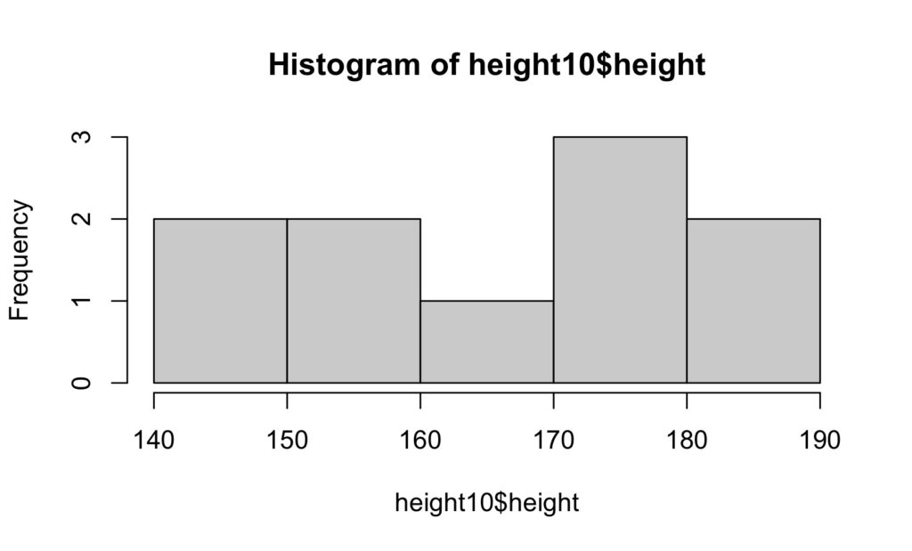
hist(tibfracture10$healingtime)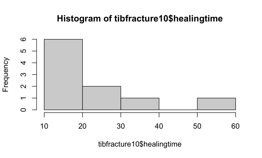
It can be seen that neither histogram particularly looks like a bell shaped curve. The healing time histogram looks very right skew (mean larger than median). Although the height histogram doesn’t look like a bell shape, there are only 10 patients and with more patients it may become bell shaped.
Graphical normality test (quantile-quantile plot)
This graphical test is probably the easiest way to test for Normality. However, it is a graphical (visual assessment) test and a p value is not obtained. The method creates a plot from the ranked samples of our data against a similar number of ranked theoretical samples from a Normal distribution. If it shows a straight line, the data is consistent with a Normal distribution. Otherwise, if the data deviates from a straight line, the distribution is not Normal.
In the R console enter:
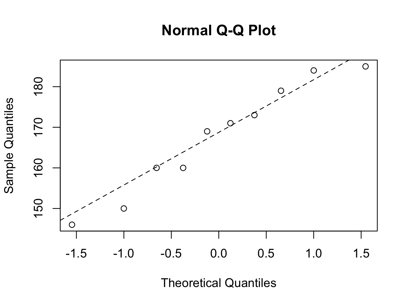
qqnorm(height10$height)
qqline(height10$height,lty=2)
The first command creates the plot and the second command draws the reference line. The parameter ‘lty=2’ is optional and creates a dotted line instead of an uninterrupted line. The data points on the qqplot are near enough the straight line and it is therefore reasonable to assume the data can be modelled with a Normal distribution.
The same for the tibial fracture healing times:
qqnorm(tibfracture10$healingtime)
qqline(tibfracture10$healingtime,lty=2)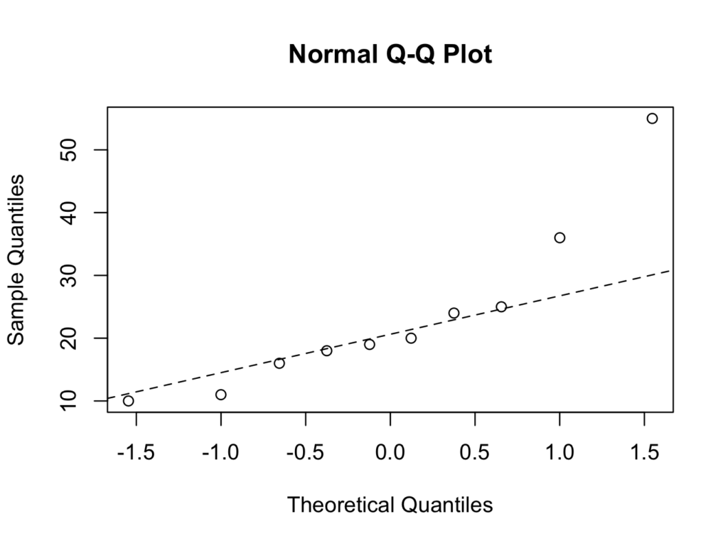
The second plot shows that the data points for tibial fracture healing time are deviating from the straight line. The fracture healing time therefore does not conform a Normal distribution (using the quantile-quantile plot method).
Shapiro-Wilk Normality test
The Shapiro-Wilk test estimates if data are consistent with a normal distribution. It is particular useful in smaller sample sizes (<2000). The null hypothesis is that the data are consistent with a normal distribution. The alternate hypothesis is that the data are not normally distributed.
To perform a Shapiro-Wilk test in R:
shapiro.test(height10$height)
    Shapiro-Wilk normality test
data:  height10$height
W = 0.9444, p-value = 0.6033

shapiro.test(tibfracture10$healingtime)
    Shapiro-Wilk normality test
data:  tibfracture10$healingtime
W = 0.8396, p-value = 0.04361
The p-value of the Shapiro-Wilk test for the height variable is 0.603 and not statisticall significant. Therefore, there is no reason to reject the null hypothesis and it is concluded that it is reasonable to regard the height data as Normally distributed.
However, the p-value for the healing time is 0.044, which is significant. Therefore, the null hypothesis is rejected in favour of the alternate hypothesis. It is concluded the data can’t be modelled with a Normal distribution. Consequently, the t-test should not be used for analysis, but non-parametric analysis should be used instead.
Kolmogorov-Smirnov Normality test
The Kolmogorov-Smirnov ‘goodness to fit’ test examines whether two datasets differ significantly. It makes no assumption on the distribution of the data and is technically speaking a non-parametric test. It can also be used to demonstrate that the data fit other distributions (outside the scope of this book). However, because the Kolmogorov-Smirnov test is more general, it tends to be less powerful (larger numbers are required to note a difference). The test is especially useful in larger sample sizes (> 50). The null hypothesis is that the data follow the specified distribution and the alternate hypothesis is that the data are not from the same distribution. To test whether the height data conform a Normal distribution, enter in the command window:
ks.test(height10$height,"pnorm",mean=mean(height10$height),sd=sd(height10$height))

	Asymptotic one-sample Kolmogorov-Smirnov test

data:  height10$height
D = 0.13841, p-value = 0.9909
alternative hypothesis: two-sided

Warning message:
In ks.test.default(height10$height, "pnorm", mean = mean(height10$height),  :
  ties should not be present for the one-sample Kolmogorov-Smirnov test
The Kolmogorov-Smirnov test compares the height data with a Normal distribution (“pnorm”) that has a mean and standard deviation that is the same as the height data (mean =mean(height10$height) and sd=sd(height10$height)). The p -value is 0.9909 and there is no reason to reject the null hypothesis (there is no difference between the height data and a Normal distribution with the same mean and standard deviation). It can be concluded that the height conforms a Normal distribution using the Kolmogorov-Smirnov test.
The output does state that a correct p-value can’t be computed with ties (the same values in the data). This is because two of the ten patients have a height of 160 cm. This can easily be overcome by introducing a greater precision into the data
height=c(184,146,169,185,160,173,179,171,160.001,150)Now, the test gives a more accurate p-value:
ks.test(height,"pnorm",mean=mean(height),sd=sd(height))
    One-sample Kolmogorov-Smirnov test
data:  height
D = 0.1384, p-value = 0.9769
alternative hypothesis: two-sided
Please note that a new variable height has been declared that is different from the height variable in the height10 data frame. As a result, only height is entered as argument for the function and not height10$height.
To test the fracture healing time data with the Kolmogorov-Smirnov test:
ks.test(tibfracture10$healingtime,"pnorm",mean=mean(tibfracture10$healingtime),sd=sd(tibfracture10$healingtime))
    One-sample Kolmogorov-Smirnov test
data:  tibfracture10$healingtime
D = 0.2524, p-value = 0.4723
alternative hypothesis: two-sided
On the basis of the Kolmogorov-Smirnov test, the null hypothesis (there is no difference between the healing time data and a Normal distribution with a the same mean and standard deviation) can’t be rejected. It may be concluded that the data can be reasonably modelled with a Normal distribution. However, the graphical method and the Shapiro-Wilk test have shown that the healing time is does not conform a Normal distribution. This illustrates the lesser statistical power of the Kolmogorov-Smirnov test, especially in smaller sample sizes.
Overall, it can be concluded that it is reasonable to model height with a Normal distribution, but not the healing time.