A radar or spider-web plot is a great way to visualise multivariate data when there are three or more continuous variables and several groups (categorical data). In this example data are first prepared and then two methods to create a radar plot will be described.
Preparation of the data
Download and open the tests.rda dataset for this example and open it in R. The data set contains the results of 5 tests as a classifier for infection. The gold standard for infection is indicated by the variable ‘standard’. All variables are binary (0, 1) and data that are not available are indicated by ‘NA’. The data can be shown by:
tests
   test1 test2 test3 test4 test5 standard
1      0     1     0     0     0        0
2      1    NA    NA    NA     0        0
.....
.....
55     1     0     1     0     0        0
It is straightforward to create a confusion table that compare the classifier to the gold standard:
test1 <- table(tests$test1, tests$standard)
test2 <- table(tests$test2, tests$standard)
test3 <- table(tests$test3, tests$standard)
test4 <- table(tests$test4, tests$standard)
test5 <- table(tests$test5, tests$standard)
The show the confusion table for test 3:
test3
   0  1
  0 35  2
  1 10  4
The positive predictive value, negative predictive value, sensitivity, specificity and accuracy can be found using the epiR package1. Unfortunately, the data in the confusion table is in the wrong order to be inserted into the epi.tests function of the epiR package. To change the order of the matrix:
matrix_test1 <-matrix(c(test1[2,2],test1[1,2],test1[2,1],test1[1,1]), ncol = 2)
matrix_test2 <-matrix(c(test2[2,2],test2[1,2],test2[2,1],test2[1,1]), ncol = 2)
matrix_test3 <-matrix(c(test3[2,2],test3[1,2],test3[2,1],test3[1,1]), ncol = 2)
matrix_test4 <-matrix(c(test4[2,2],test4[1,2],test4[2,1],test4[1,1]), ncol = 2)
matrix_test5 <-matrix(c(test5[2,2],test5[1,2],test5[2,1],test5[1,1]), ncol = 2)
To show, for example, the matrix of test 3:
matrix_test3
     [,1] [,2]
[1,]    4   10
[2,]    2   35
To summarise the positive predictive value, negative predictive value, sensitivity, specificity and accuracy using the epiR package2, one large matrix (called overall) can be build after the epiR package has been loaded:
library(epiR)

overall <- matrix(c(
epi.tests(matrix_test1)$detail$est[epi.tests(matrix_test1)$detail$statistic == "pv.pos"],
epi.tests(matrix_test1)$detail$est[epi.tests(matrix_test1)$detail$statistic == "pv.neg"],
epi.tests(matrix_test1)$detail$est[epi.tests(matrix_test1)$detail$statistic == "se"],
epi.tests(matrix_test1)$detail$est[epi.tests(matrix_test1)$detail$statistic == "sp"],
epi.tests(matrix_test1)$detail$est[epi.tests(matrix_test1)$detail$statistic == "diag.ac"],
epi.tests(matrix_test2)$detail$est[epi.tests(matrix_test2)$detail$statistic == "pv.pos"],
epi.tests(matrix_test2)$detail$est[epi.tests(matrix_test2)$detail$statistic == "pv.neg"],
epi.tests(matrix_test2)$detail$est[epi.tests(matrix_test2)$detail$statistic == "se"],
epi.tests(matrix_test2)$detail$est[epi.tests(matrix_test2)$detail$statistic == "sp"],
epi.tests(matrix_test2)$detail$est[epi.tests(matrix_test2)$detail$statistic == "diag.ac"],
epi.tests(matrix_test3)$detail$est[epi.tests(matrix_test3)$detail$statistic == "pv.pos"],
epi.tests(matrix_test3)$detail$est[epi.tests(matrix_test3)$detail$statistic == "pv.neg"],
epi.tests(matrix_test3)$detail$est[epi.tests(matrix_test3)$detail$statistic == "se"],
epi.tests(matrix_test3)$detail$est[epi.tests(matrix_test3)$detail$statistic == "sp"],
epi.tests(matrix_test3)$detail$est[epi.tests(matrix_test3)$detail$statistic == "diag.ac"],
epi.tests(matrix_test4)$detail$est[epi.tests(matrix_test4)$detail$statistic == "pv.pos"],
epi.tests(matrix_test4)$detail$est[epi.tests(matrix_test4)$detail$statistic == "pv.neg"],
epi.tests(matrix_test4)$detail$est[epi.tests(matrix_test4)$detail$statistic == "se"],
epi.tests(matrix_test4)$detail$est[epi.tests(matrix_test4)$detail$statistic == "sp"],
epi.tests(matrix_test4)$detail$est[epi.tests(matrix_test4)$detail$statistic == "diag.ac"],
epi.tests(matrix_test5)$detail$est[epi.tests(matrix_test5)$detail$statistic == "pv.pos"],
epi.tests(matrix_test5)$detail$est[epi.tests(matrix_test5)$detail$statistic == "pv.neg"],
epi.tests(matrix_test5)$detail$est[epi.tests(matrix_test5)$detail$statistic == "se"],
epi.tests(matrix_test5)$detail$est[epi.tests(matrix_test5)$detail$statistic == "sp"],
epi.tests(matrix_test5)$detail$est[epi.tests(matrix_test5)$detail$statistic == "diag.ac"]),
ncol = 5)
To show the matrix, just call the object:
overall
          [,1]      [,2]      [,3]      [,4]      [,5]
[1,] 0.1724138 0.2500000 0.2857143 0.6000000 0.8000000
[2,] 0.9615385 0.9736842 0.9459459 0.9772727 0.9795918
[3,] 0.8333333 0.7500000 0.6666667 0.7500000 0.8000000
[4,] 0.5102041 0.8043478 0.7777778 0.9555556 0.9795918
[5,] 0.5454545 0.8000000 0.7647059 0.9387755 0.9629630
Apply collumn and row names and round the values:
colnames(overall) <- c('Test1','Test2','Test3','Test4','Test5')
rownames(overall) <- c('PPV', 'NPV', 'Sens', 'Spec', 'Acc')
round(overall*100,0)
     Test1 Test2 Test3 Test4 Test5
PPV     17    25    29    60    80
NPV     96    97    95    98    98
Sens    83    75    67    75    80
Spec    51    80    78    96    98
Acc     55    80    76    94    96
The matrix can be transposed (t) and converted to a data frame, called radar, for subsequent analysis:
radar <- t(round(overall*100,0))
radar <- as.data.frame(radar)
radar
      PPV NPV Sens Spec Acc
Test1  17  96   83   51  55
Test2  25  97   75   80  80
Test3  29  95   67   78  76
Test4  60  98   75   96  94
Test5  80  98   80   98  96
Two Methods to create a radar plot will be described:
- Using the fmsb package3(easier, but less versatile)
- Using function as provided by LePennec4 using the ggplot2 package5
Method 1:
Make sure the fmsb6 package is loaded and create a simple radar plot:
library(fmsb)
radarchart(radar, maxmin = F)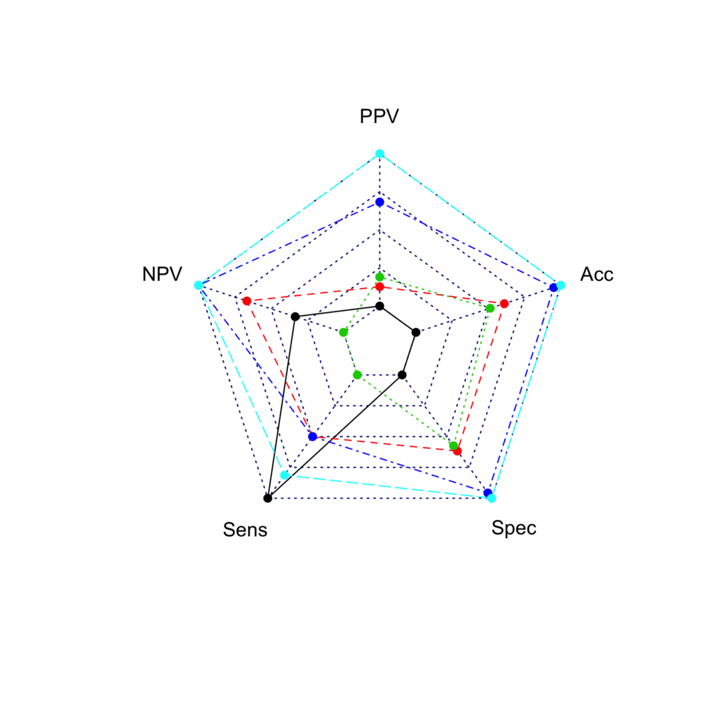
The add maximum (100) and minimum (0) values to the plot, they need to be inserted to the first and second row of the data frame respectively:
radar2 <- rbind(rep(100,5) , rep(0,5) , radar)
radarchart(radar2)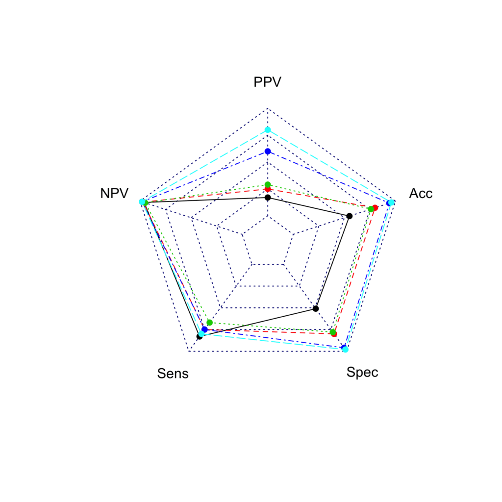
A better looking plot can be obtained by setting the arguments as per the manual of the package:
colours <- c( 'tomato','orchid','grey','gold', 'seagreen')

radarchart(radar, axistype=1 , maxmin=F, pcol=colours, plwd=4, plty=1,
 cglcol="grey", cglty=1, axislabcol="black", cglwd=0.8, vlcex=0.8)
legend(x=0.7, y=1.2, legend = rownames(radar), bty = "n", pch=20, col=colours, text.col = "grey", cex=1.2, pt.cex=3)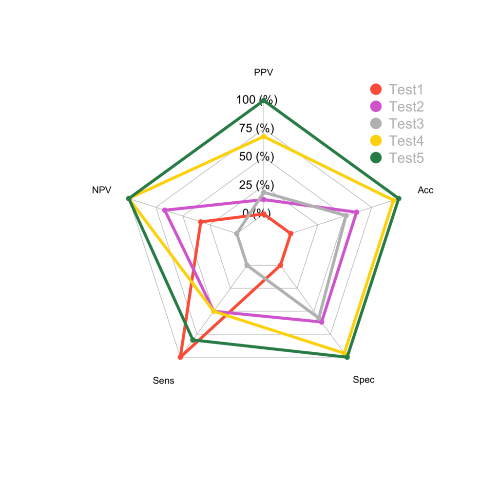
Method 2:
This method is more versatile, but requires more packages to be loaded. Plots are created using the ggplot2 package7 and a function from LePennec8.
Make sure the required packages , including reshape29, are loaded:
library(reshape2)
library(ggplot2)
Have a look at the data frame again:
radar
      PPV NPV Sens Spec Acc
Test1  17  96   83   51  55
Test2  25  97   75   80  80
Test3  29  95   67   78  76
Test4  60  98   75   96  94
Test5  80  98   80   98  96
The data frame needs to contain a varaible that contains the test; therefore define a new data frame and call it radar3:
test <- c("Test 1", "Test 2", "Test 3", "Test 4", "Test 5")
radar3 <- cbind(test, radar)
radar3
        test PPV NPV Sens Spec Acc
Test1 Test 1  17  96   83   51  55
Test2 Test 2  25  97   75   80  80
Test3 Test 3  29  95   67   78  76
Test4 Test 4  60  98   75   96  94
Test5 Test 5  80  98   80   98  96
Now melt the data using the reshape2 package10:
radar4 <- melt(radar3)
radar4
     test variable value
1  Test 1      PPV    17
2  Test 2      PPV    25
.....
.....
25 Test 5      Acc    96
and give collumn names:
colnames(radar4) <- c('Test', 'Descript', 'Value')
radar4
     Test Descript Value
1  Test 1      PPV    17
2  Test 2      PPV    25
.....
.....
25 Test 5 Acc 96LePennec11 has defined a function that creates radar charts with the ggplot2 package. Load the function:
coord_radar <- function (theta = c("x", "y"), start = 0, direction = 1) {
theta <- match.arg(theta)
r <- if (theta == "x") "y" else "x"
ggproto(
"CoordRadar", CoordPolar,
theta = theta,
r = r,
start = start,
direction = sign(direction),
is_linear = function(coord) TRUE
)
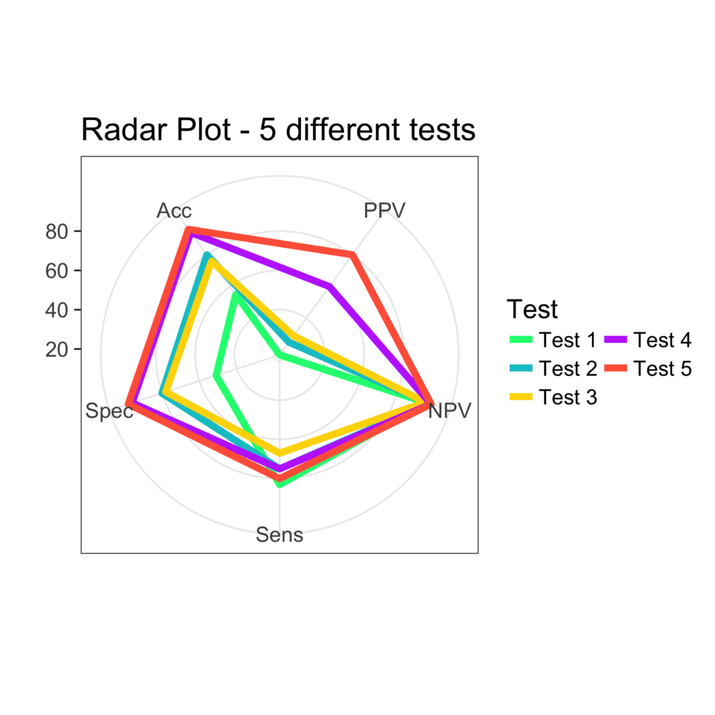
}Finally, build the plot using the ggplot2 package:
ggplot(radar4, aes(x = Descript, y = Value)) +
geom_polygon(aes(group = Test, color = Test), fill = NA, size = 2, show.legend = FALSE) +
geom_line(aes(group = Test, color = Test), size = 2) +
xlab("") + ylab("") +
guides(color = guide_legend(ncol=2)) +
scale_color_manual(values = c('springgreen', 'turquoise3', 'gold', 'darkorchid1', 'tomato')) +
coord_radar() +
ggtitle('Radar Plot - 5 different tests') +
theme_bw(base_size = 16)