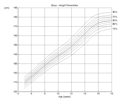
Below are typical growth curves for boys:
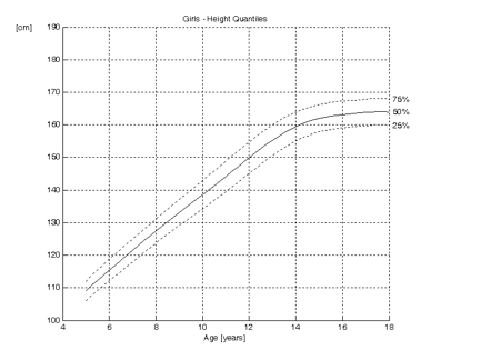
And Girls:
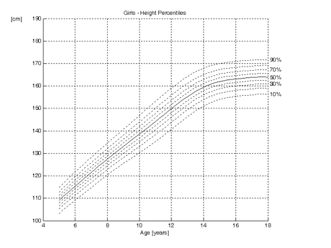
The curves show the height as function of the age for boys and girls.
The dotted lines are the percentiles. They indicate the proportion of children that are below a certain height. Ten per cent of the children are below the 10th percentile in height and consequently 90% are above it. Similarly, 30 per cent of the children are below the 30th percentile and 70 per cent above it. Also, 70 per cent are below the 70th percentile and 30 per cent above it.
The 50th percentile is shown as a solid line. Indeed, 50 per cent of the children are taller than the 50th percentile and 50 per cent shorter. It can be demonstrated that height is normally distributed. Therefore, in growth curves, the 50th percentile (P50) is the same as the mean (average), mode and the median.
P50 = mean = mode = median
It can be read from the growth curves above, that the mean final height for boys is approximately 176 cm, whilst this is 164 cm for girls. Twelve year old girls are on average 150 cm tall, whilst boys this age are approximately 148 cm. From these curves, it can also be seen that girls reach maturity earlier than boys. The curve for girls reaches a plateau at 15 years of age, whilst this is approximately 17 years for boys.
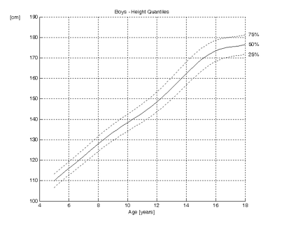
Quantiles are similar to percentiles. As the name implies, quantiles divide the data in four groups. The first quantile is at 25%, the second at 50%, the third at 75% and the fourth at 100%. So, the 25th percentile is the same as the first quantile. The 2nd quantile line is the same as the 50th percentile, the median, mode and median.
P50 = mean = mode = median = 2nd quantile
Growth curves with quantiles are shown below; only the 1st, 2nd and 3rd quantiles are shown:
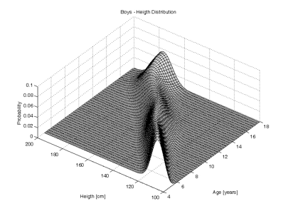
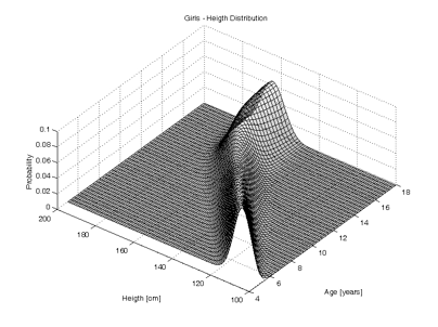
As stated previously, height is normally distributed. At any particular age, the percentiles show a Gaussian or bell shaped curve. The growth charts are a continuum of Gaussian curves. This is shown three dimensionally below:
In normally distributed data, 68.27% of the data lie in an interval plus or minus one standard deviation from the mean. Similarly 95.45% of the data lie in an interval plus or minus twice the standard deviation and 99.73% of the data within an interval plus or minus three times the standard deviation.
Or:
Mean ± 1 × SD = 68.27 %
Mean ± 2 × SD = 95.45 %
Mean ± 3 × SD = 99.73 %
To ‘translate’ this into percentiles:
One standard deviation about the mean:
68.27 % about the mean (P50) is the interval between
50 – (68.27 / 2) = 50 – 34.135 = 15.865 » 16th percentile
and
50 + (68.27 / 2) = 50 + 34.135 = 84.135 » 84th percentile
Similarly, two standard deviations about the mean:
50 – (95.45 / 2) = 50 – 47.725 = 2.275 » 2nd percentile
and
50 + (95.45 / 2) = 50 + 47.725 = 97.725 » 98th percentile
And three:
50 – (99.73 / 2) = 50 – 49.865 = 0.135 » 0.1th percentile
and
50 + (99.73 / 2) = 50 + 49.865 = 99.865 » 99.9th percentile
In summary:
Mean ± 1 × SD = 68.27 % : between 16th and 84th percentile
Mean ± 2 × SD = 95.45 % : between 2nd and 98th percentile
Mean ± 3 × SD = 99.73 % : between 0.1th and 99.9th percentile
In R:
Sample data abstracted from the UK 1990 growth data are provided in malegrowth.rda. Load the data and show (the data frame is called ‘male’):
load("~/Desktop/malegrowth.rda")
male
year X0.4th X2nd X9th X25th X50th X75th X91st X98th
2 0 45.743 46.938 48.362 49.693 51.04 52.387 53.718 55.142
3 1 68.875 70.372 72.156 73.823 75.51 77.197 78.864 80.648
4 2 78.607 80.456 82.658 84.716 86.80 88.884 90.942 93.144
5 3 85.749 87.929 90.526 92.953 95.41 97.867 100.294 102.891
6 4 91.596 94.054 96.982 99.719 102.49 105.261 107.998 110.926
7 5 97.584 100.292 103.520 106.536 109.59 112.644 115.660 118.888
8 6 103.048 105.954 109.417 112.654 115.93 119.206 122.443 125.906
9 7 108.222 111.308 114.985 118.421 121.90 125.379 128.815 132.492
10 8 113.324 116.601 120.507 124.156 127.85 131.544 135.193 139.099
11 9 117.901 121.370 125.505 129.369 133.28 137.191 141.055 145.190
12 10 121.992 125.691 130.100 134.219 138.39 142.561 146.680 151.089
13 11 125.735 129.714 134.455 138.885 143.37 147.855 152.285 157.026
14 12 129.285 133.588 138.717 143.509 148.36 153.211 158.003 163.132
15 13 133.968 138.661 144.253 149.479 154.77 160.061 165.287 170.879
16 14 140.357 145.321 151.236 156.764 162.36 167.956 173.484 179.399
17 15 147.385 152.248 158.043 163.458 168.94 174.422 179.837 185.632
18 16 153.208 157.761 163.187 168.257 173.39 178.523 183.593 189.019
19 17 156.810 161.121 166.259 171.060 175.92 180.780 185.581 190.719
20 18 158.501 162.695 167.692 172.362 177.09 181.818 186.488 191.485
21 19 158.779 162.953 167.927 172.575 177.28 181.985 186.633 191.607
22 20 158.861 163.030 167.998 172.640 177.34 182.040 186.682 191.650
23 21 159.185 163.333 168.275 172.894 177.57 182.246 186.865 191.807
24 22 159.582 163.704 168.615 173.204 177.85 182.496 187.085 191.996
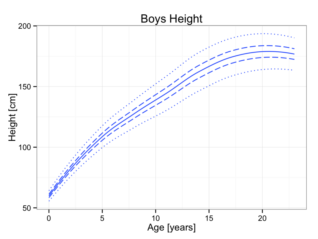
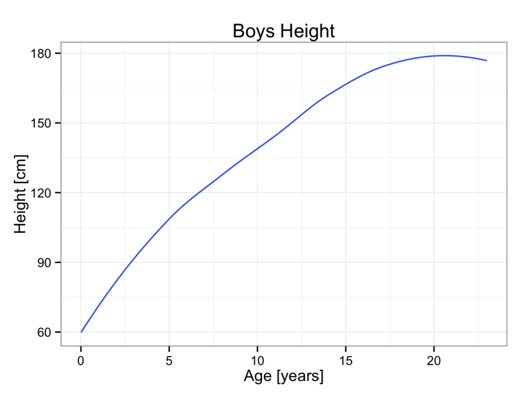
25 23 160.112 164.200 169.071 173.622 178.23 182.838 187.389 192.260Plot builder can be used to construct a growth chart based on these data using the geom_smooth (Loess) best fit lines. Each line is added to a plot:
male_growth <- male %>%
ggplot(aes(x = year,y = X50th)) +
geom_smooth(,se = FALSE) +
ggtitle(label = 'Boys Height') +
xlab(label = 'Age [years]') +
ylab(label = 'Height [cm]') +
theme_bw()

male_growth
This will create a plot with the mean height for boys:
It is easy to add the 2nd, 98th, 25th and 75th percentiles:
male_growth <- male_growth +
geom_smooth(aes(x=year, y=X2nd), data=male, linetype=3, se=FALSE) +
geom_smooth(aes(x=year, y=X98th), data=male, linetype=3, se=FALSE) +
geom_smooth(aes(x=year, y=X25th), data=male, linetype=5, se=FALSE) +
geom_smooth(aes(x =year, y=X75th), data=male, linetype=5, se=FALSE)

male_growth