Linear Discriminant Analysis

Linear Discriminant Analysis(LDA) is a linear transformation technique of supervised machine learning (there needs to be a classifier). The aim of the technique is to find a linear combination of variables that separates the classifier variables as much as possible.

To illustrate the method, R’s build in data set “iris” is used. The iris data set contains the sepal and petal length and width of three different types of iris plants: Setosa, Versicolor and Virginica. Have a look at the iris data set:

head(iris)
Sepal.Length Sepal.Width Petal.Length Petal.Width Species
1 5.1 3.5 1.4 0.2 setosa
2 4.9 3.0 1.4 0.2 setosa
3 4.7 3.2 1.3 0.2 setosa
4 4.6 3.1 1.5 0.2 setosa
5 5.0 3.6 1.4 0.2 setosa
6 5.4 3.9 1.7 0.4 setosa
str(iris)
‘data.frame': 150 obs. of 5 variables:
$ Sepal.Length: num 5.1 4.9 4.7 4.6 5 5.4 4.6 5 4.4 4.9 …
$ Sepal.Width : num 3.5 3 3.2 3.1 3.6 3.9 3.4 3.4 2.9 3.1 …
$ Petal.Length: num 1.4 1.4 1.3 1.5 1.4 1.7 1.4 1.5 1.4 1.5 …
$ Petal.Width : num 0.2 0.2 0.2 0.2 0.2 0.4 0.3 0.2 0.2 0.1 …
$ Species : Factor w/ 3 levels “setosa”,”versicolor”,..: 1 1 1 1 1 1 1 1 1 1 …

Load the MASS package:

library(MASS)

And perform linear discriminant analysis:

lda_iris <- lda(iris$Species ~ iris[,1] + iris[,2] + iris[,3] + iris[,4])
lda_iris
Call:
lda(iris$Species ~ iris[, 1] + iris[, 2] + iris[, 3] + iris[, 
    4])

Prior probabilities of groups:
    setosa versicolor  virginica 
 0.3333333  0.3333333  0.3333333 

Group means:
           iris[, 1] iris[, 2] iris[, 3] iris[, 4]
setosa         5.006     3.428     1.462     0.246
versicolor     5.936     2.770     4.260     1.326
virginica      6.588     2.974     5.552     2.026

Coefficients of linear discriminants:
                 LD1         LD2
iris[, 1]  0.8293776 -0.02410215
iris[, 2]  1.5344731 -2.16452123
iris[, 3] -2.2012117  0.93192121
iris[, 4] -2.8104603 -2.83918785

Proportion of trace:
   LD1    LD2 
0.9912 0.0088

Now use the model to predict the species of each plant:

lda_iris_predict <- predict(lda_iris, iris[,1:4])

Attach this predicted variable (stored in lda_iris_predict$class) to the original iris data frame as a new variable called Predict and have a look at the top (head) of the data frame:

iris$Predict <- lda_iris_predict$class
head(iris)
  Sepal.Length Sepal.Width Petal.Length Petal.Width Species Predic
1          5.1         3.5          1.4         0.2  setosa  setosa
2          4.9         3.0          1.4         0.2  setosa  setosa
3          4.7         3.2          1.3         0.2  setosa  setosa
4          4.6         3.1          1.5         0.2  setosa  setosa
5          5.0         3.6          1.4         0.2  setosa  setosa
6          5.4         3.9          1.7         0.4  setosa  setosa

The values of the discriminant functions can be found by:

lda_iris_predict$x[,1] # values for the first discriminant function
         1          2          3          4          5          6          7          8          9         10         11         12         13         14         15 
 8.0617998  7.1286877  7.4898280  6.8132006  8.1323093  7.7019467  7.2126176  7.6052935  6.5605516  7.3430599  8.3973865  7.2192969  7.3267960  7.5724707  9.8498430 
.....
.....
       136        137        138        139        140        141        142        143        144        145        146        147        148        149        150 
-6.7967163 -6.5244960 -4.9955028 -3.9398530 -5.2038309 -6.6530868 -5.1055595 -5.5074800 -6.7960192 -6.8473594 -5.6450035 -5.1795646 -4.9677409 -5.8861454 -4.6831543 

lda_iris_predict$x[,2] # values for the second discriminant function
           1            2            3            4            5            6            7            8            9           10           11           12           13 
-0.300420621  0.786660426  0.265384488  0.670631068 -0.514462530 -1.461720967 -0.355836209  0.011633838  1.015163624  0.947319209 -0.647363392  0.109646389  1.072989426 
 .....
.....
         144          145          146          147          148          149          150 
-1.460686950 -2.428950671 -1.677717335  0.363475041 -0.821140550 -2.345090513 -0.332033811

How good were the predictions? Just create a confusion table of the classifier (Species) agains the predictor (Predict):

table(iris$Species, iris$Predict)

	Setosa	Versicolor	Virginica
Setosa	50	0	0
Versicolor	0	48	2
Virginica	0	1	49

So, all Setosa species were predicted correctly. Two Versicolor species were incorrectly labelled as Virginica and one Virginica was incorrectly labelled as Versicolor. Consequently, the accuracy is:

$Acc = \frac{50 + 48 + 49}{150} = 98\% $

To plot the data in ggplot:

iris_lda_df <- data.frame(first = lda_iris_predict$x[,1], 
second = lda_iris_predict$x[,2], Species = iris$Species, 
Predict = iris$Predict)

ggplot(iris_lda_df, aes(x = first, y = second, colour = Species, 
shape = Predict)) +
  geom_point(size = 4, alpha = 0.8) +
  ggtitle("Linear Discriminant Analysis") +
  scale_x_continuous("First Discriminant Function") +
  scale_y_continuous("Second Discriminant Function") +
  theme_bw()

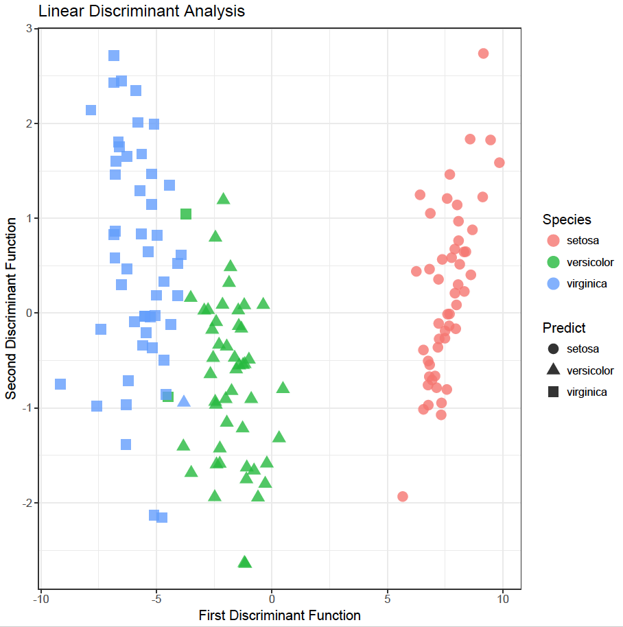
The plot shows the separation obtained and the classification (actual and predicted). The two green squares were predicted as Virginica, but are actually Versicolor species. Similarly, the blue triangle was predicted as Versicolor but was actually a Virginica species. Overall, a very satisfactory model!