A decision tree plot can be useful to visualise decision rules for categorical or continuous outcome variables. A popular package to create decision trees in R is rpart1. In addition, there is a separate package to produce plots with rpart; rpart.plot2. Both packages should be installed.
Binary (categorical) outcome
The rpart package 3 contains a data frame with information about patients with kyphosis. To view the first 6 observations:
library(rpart)
head(kyphosis)
  Kyphosis Age Number Start
1   absent  71      3     5
2   absent 158      3    14
3  present 128      4     5
4   absent   2      5     1
5   absent   1      4    15
6   absent   1      2    16
The data frame contains 4 variables (str stands for structure):
str(kyphosis)
'data.frame': 81 obs. of 4 variables:
 $ Kyphosis: Factor w/ 2 levels "absent","present": 1 1 2 1 1 1 1 1 1 2 ...
 $ Age : int 71 158 128 2 1 1 61 37 113 59 ...
 $ Number : int 3 3 4 5 4 2 2 3 2 6 ...
 $ Start : int 5 14 5 1 15 16 17 16 16 12 ...
The variable ‘Kyphosis’ is categorical and is either ‘absent’ or ‘present’. The variable ‘Number’ is integer and shows the number of vertebrae involved. The variable ‘Start’ is the highest vertebra.
To create a decision tree (machine learning) plot is straight forward:
model <- rpart(Kyphosis ~ Age + Number + Start, data = kyphosis, method = 'class')The variable to the left of the tilde (~) is the outcome (response) variable and the variables to the right of the tilde are the explanatory variables. To show the model:
model
n= 81

node), split, n, loss, yval, (yprob)
      * denotes terminal node

 1) root 81 17 absent (0.79012346 0.20987654)
   2) Start>=8.5 62  6 absent (0.90322581 0.09677419)
     4) Start>=14.5 29  0 absent (1.00000000 0.00000000) *
     5) Start< 14.5 33  6 absent (0.81818182 0.18181818)
      10) Age< 55 12  0 absent (1.00000000 0.00000000) *
      11) Age>=55 21  6 absent (0.71428571 0.28571429)
        22) Age>=111 14  2 absent (0.85714286 0.14285714) *
        23) Age< 111 7  3 present (0.42857143 0.57142857) *
   3) Start< 8.5 19  8 present (0.42105263 0.57894737) *
A plot is more informative:
plot(model)
text(model)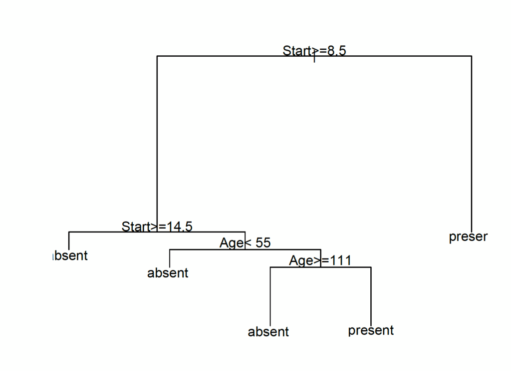
Although it is possible to reduce the text size (with cex = 0.8), the plot doesn’t look very good. However, there is an additional package rpart.plot4 for enhanced graphics.
library(rpart.plot)
rpart.plot(model)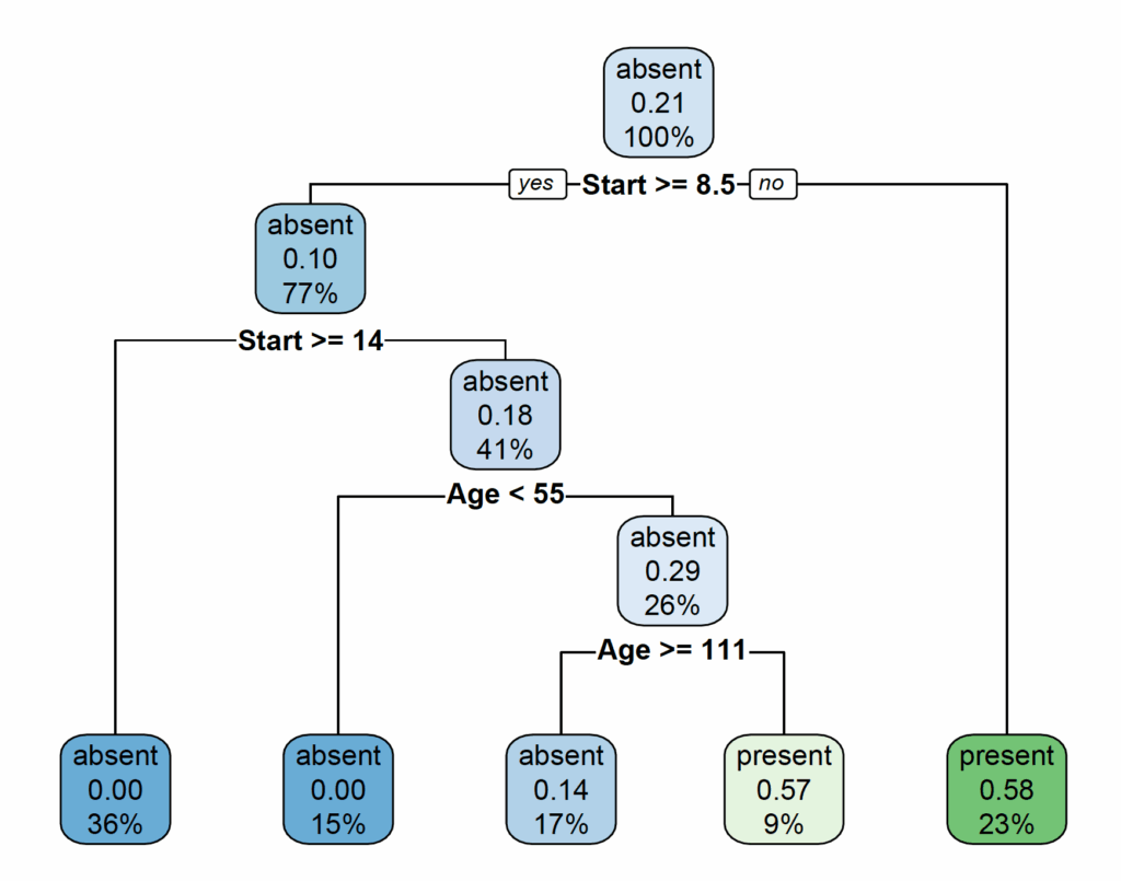
Continuous outcome variable (regression)
The rpart package also contains a data frame cu.summary with information about different cars. To show the data frame’s first six observations as well as its structure:
library(rpart)
head(cu.summary)
                Price Country Reliability Mileage  Type
Acura Integra 4 11950   Japan Much better      NA Small
Dodge Colt 4     6851   Japan        <NA>      NA Small
Dodge Omni 4     6995     USA  Much worse      NA Small
Eagle Summit 4   8895     USA      better      33 Small
Ford Escort   4  7402     USA       worse      33 Small
Ford Festiva 4   6319   Korea      better      37 Small

str(cu.summary)
'data.frame':	117 obs. of  5 variables:
 $ Price      : num  11950 6851 6995 8895 7402 ...
 $ Country    : Factor w/ 10 levels "Brazil","England",..: 5 5 10 10 10 7 5 6 6 7 ...
 $ Reliability: Ord.factor w/ 5 levels "Much worse"<"worse"<..: 5 NA 1 4 2 4 NA 5 5 2 ...
 $ Mileage    : num  NA NA NA 33 33 37 NA NA 32 NA ...
 $ Type       : Factor w/ 6 levels "Compact","Large",..: 4 4 4 4 4 4 4 4 4 4 ...
To predict the car’s mileage from Price, Country, Reliability and Type (using analysis of variance: anova):
model2 <- rpart(Mileage ~ Price + Country + Reliability + Type, method="anova", data=cu.summary)
plot(model2)
text(model2)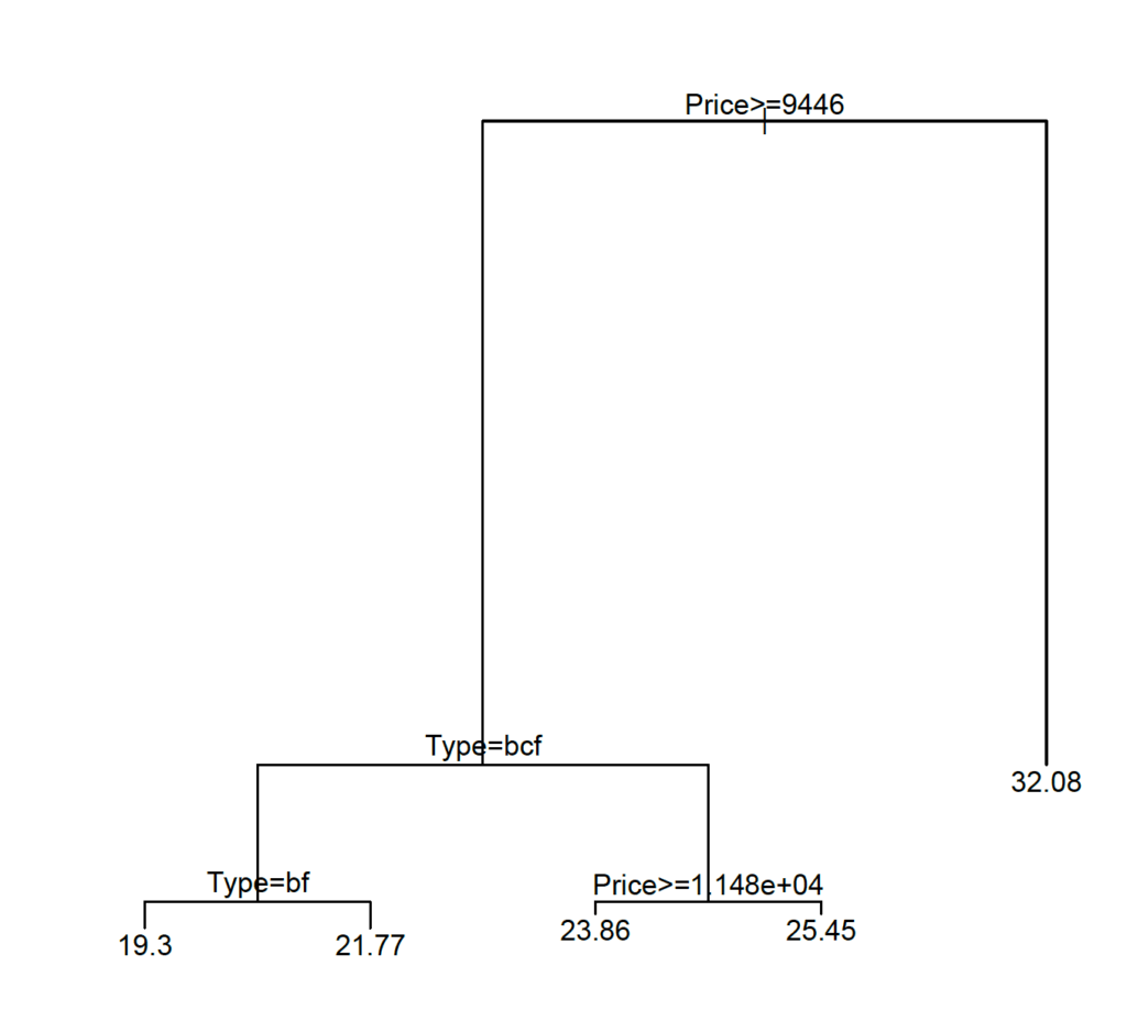
Or for a nicer plot:
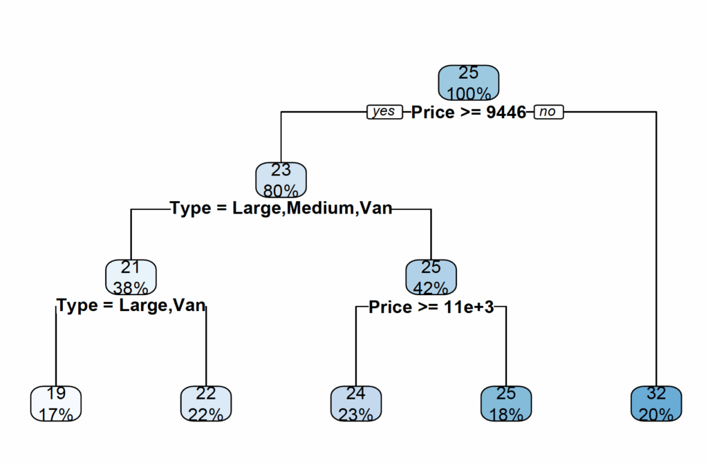
library(rpart.plot)
rpart.plot(model2)