1. Using <= 16 weeks as ‘cut off’ point, indicate patients were fracture healing had occurred within 16 weeks by ‘-‘ and patients who took longer than 16 weeks to unite by ‘+’. In the smoking group, there were 7 out of 12 patients were fracture union was in excess of 16 weeks. Whilst In the non smokers, there was only 1 out of 8 patients were the fracture took longer than 16 weeks to unite. Is this due to chance?We formulate a null hypothesis; there is no difference in fracture healing time between smokers and non smokers and test this hypothesis. Using a two sided sign test the probability is:
P > 5%, therefore NOT statistically significant. The null hypothesis can therefore NOT be rejected. We conclude that we were unable to demonstrate a difference in fracture healing time between smokers and non smokers.
The same result is obtained if the calculation is performed in R:
binom.test(1,8)

	Exact binomial test

data:  1 and 8
number of successes = 1, number of trials = 8, p-value = 0.07031
alternative hypothesis: true probability of success is not equal to 0.5
95 percent confidence interval:
 0.003159724 0.526509671
sample estimates:
probability of success
                 0.125
2. Using the Chi Square test, we need to first construct a table with the observed frequencies and the expected frequencies:
| Smoker Observed | Smoker Expected | Non Smoker Observed | Non Smoker Expected | Total | |
|---|---|---|---|---|---|
| <= 16 weeks | 5 | 12×12/20 = 7.2 | 7 | 8×12/20 = 4.8 | 12 |
| > 16 weeks | 7 | 12×8/20 = 4.8 | 1 | 8×8/20 = 3.2 | 8 |
| 12 | 12 | 8 | 8 | 20 |
The observed frequency table has two rows and two columns. Therefore, there is 1 degree of freedom (r-1)×(c-1). Using the Chi Square distribution table we can see that there is statistical significance (p < 5%). However, not all prerequisites of the Chi Square test have been met as the expected frequencies are not above 5. It would therefore be more appropriate to use the Yates continuity correction (should be used if the expected frequencies are below 10) or the Fisher Exact test (if expected frequencies are below 5). These tests are performed below in R.
First without continuity correction:
data<-matrix(c(5,7,7,1),nrow=2)
chisq.test(data,correct=FALSE)

    Pearson's Chi-squared test

data:  data
X-squared = 4.2014, df = 1, p-value = 0.04039

Warning message:
In chisq.test(data, correct = FALSE) :
  Chi-squared approximation may be incorrect
Obviously, R calculates the same result. The computer calculates an exact p-value, suggesting significance. However, the expected frequencies are below 5 and it is inappropriate to use the Chi Square test. To show the expected frequencies:
chisq.test(data,correct=FALSE)$expected
     [,1] [,2]
[1,]  7.2  4.8
[2,]  4.8  3.2
Warning message:
In chisq.test(data, correct = FALSE) :
  Chi-squared approximation may be incorrect
If the expected frequencies are below 10, Yates continuity correction should be used:
chisq.test(data,correct=TRUE)

    Pearson's Chi-squared test with Yates' continuity correction

data:  data
X-squared = 2.5087, df = 1, p-value = 0.1132

Warning message:
In chisq.test(data, correct = TRUE) :
  Chi-squared approximation may be incorrect
So, the Chi Square test with Yates continuity correction is insignificant! If the expected frequencies are below 5 however, a Fisher Exact test would be more appropriate:
fisher.test(data)
     Fisher's Exact Test for Count Data

data:  data
p-value = 0.06967
alternative hypothesis: true odds ratio is not equal to 1
95 percent confidence interval:
 0.001993953 1.370866340
sample estimates:
odds ratio
 0.1148794
Again, the result is insignificant.
3. To perform a Wilcoxon test in R:
wilcox.test(smokers$Time~smokers$Group,correct=FALSE)

    Wilcoxon rank sum test

data:  smokers$Time by smokers$Group
W = 26.5, p-value = 0.0949
alternative hypothesis: true location shift is not equal to 0

Warning message:
In wilcox.test.default(x = c(10L, 10L, 11L, 12L, 15L, 15L, 16L,  :
  cannot compute exact p-value with ties
The Wilcoxon test is insignificant, again failing to demonstrate a difference.
4. Normality will be tested using three methods; a quantile quantile plot, a Shapiro-Wilk test and a Kolmogorov-Smirnov test.
To create a quantile quantile plot for both groups:
qqnorm(smokers$Time)
qqline(smokers$Time)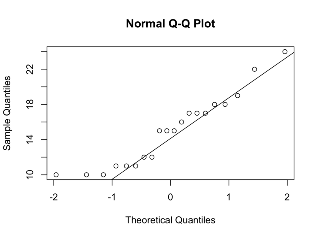
For only the smokers:
qqnorm(smokers$Time[which(smokers$Group=='Smoker')])
qqline(smokers$Time[which(smokers$Group=='Smoker')])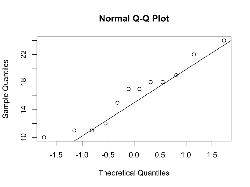
qqnorm(smokers$Time[which(smokers$Group=='Non Smoker')])
qqline(smokers$Time[which(smokers$Group=='Non Smoker')])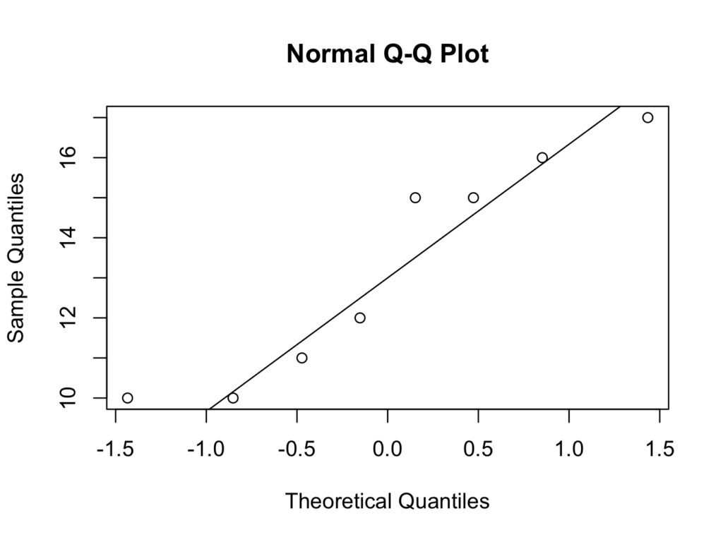
Although the numbers are small, the quantile quantile plots deviate from a straight line at the lower quantiles. Therefore, it may not be appropriate to assume the data can be modelled with a Normal distribution.
The Shapiro-Wilk test can be performed on both groups together, or separately:
shapiro.test(smokers$Time)
    Shapiro-Wilk normality test
data:  smokers$Time
W = 0.9233, p-value = 0.1148
shapiro.test(smokers$Time[which(smokers$Group=='Smoker')])
    Shapiro-Wilk normality test
data:  smokers$Time[which(smokers$Group == "Smoker")]
W = 0.9393, p-value = 0.4884
shapiro.test(smokers$Time[which(smokers$Group=='Non Smoker')])
    Shapiro-Wilk normality test
data:  smokers$Time[which(smokers$Group == "Non Smoker")]
W = 0.8837, p-value = 0.2041
The p-value is insignificant and there is no reason to reject the null hypothesis that the data is Normally distributed. It is concluded it would be reasonable to model the data with a Normal distribution.
The Kolomogorov-Smirnov test can be used to compare the variable time to a Normal distribution with the same mean and standard deviation:
ks.test(smokers$Time,"pnorm",mean=mean(smokers$Time),
   sd=sd(smokers$Time))
    One-sample Kolmogorov-Smirnov test
data:  smokers$Time
D = 0.1683, p-value = 0.6226
alternative hypothesis: two-sided
Warning message:
In ks.test(smokers$Time, "pnorm", mean = mean(smokers$Time), sd = sd(smokers$Time)) :
  ties should not be present for the Kolmogorov-Smirnov test
Or, comparing both groups:
ks.test(smokers$Time[which(smokers$Group=='Smoker')],
   smokers$Time[which(smokers$Group=='Non Smoker')])
    Two-sample Kolmogorov-Smirnov test
data:  smokers$Time[which(smokers$Group == "Smoker")] and smokers$Time[which(smokers$Group == "Non Smoker")]
D = 0.4583, p-value = 0.2656
alternative hypothesis: two-sided
Warning message:
In ks.test(smokers$Time[which(smokers$Group == "Smoker")], smokers$Time[which(smokers$Group ==  :
  cannot compute exact p-value with ties
Again, there is no reason to reject the null hypothesis and Normality is assumed on the basis of the Shapiro-Wilk and Kolmogorov-Smirnov tests.
5. The answer to question 4 suggests it is reasonable to assume Normality and therefore to use a t-test. To perform a power analsysis in R :
The mean of the Time variable is:
mean(smokers$Time)
[1] 15
The standard deviation of the Time variable is:
sd(smokers$Time)
[1] 4.091069
Delta is 10% of the mean, so delta is 1.5. The significance level is 0.05 and the power 80% (0.08):
power.t.test(sd=4.09,delta=1.5,sig.level=0.05,power=0.8)
     Two-sample t test power calculation
              n = 117.6764
          delta = 1.5
             sd = 4.09
      sig.level = 0.05
          power = 0.8
    alternative = two.sided
NOTE: n is number in *each* group
Therefore, 118 patients are required in each group (study size 236).
6. First a 2 × 2 table is constructed:
| Truth Positive | Truth Negative | ||
|---|---|---|---|
| Test Positive | 6 | 4 | 10 |
| Test Negative | 30 | 10 | 40 |
| 36 | 14 | 50 |
- True Positive: 6
- False Positive: 4
- False Negative: 30
- True Negative: 10
- ppv = 60%
- npv = 25%
- Sensitivity ≈ 17%
- Specificity ≈ 71%
- Accuracy = 32%
Or in R :
library(epiR)
Package epiR 0.9-62 is loaded
Type help(epi.about) for summary information
mat<-matrix(c(6,30,4,10),ncol=2)
mat
     [,1] [,2]
[1,]    6    4
[2,]   30   10
epi.tests(mat)
          Disease +    Disease -      Total
Test +            6            4         10
Test -           30           10         40
Total            36           14         50

Point estimates and 95 % CIs:
---------------------------------------------------------
Apparent prevalence                    0.20 (0.10, 0.34)
True prevalence                        0.72 (0.58, 0.84)
Sensitivity                            0.17 (0.06, 0.33)
Specificity                            0.71 (0.42, 0.92)
Positive predictive value              0.60 (0.26, 0.88)
Negative predictive value              0.25 (0.13, 0.41)
Positive likelihood ratio              0.58 (0.19, 1.76)
Negative likelihood ratio              1.17 (0.81, 1.68)
---------------------------------------------------------