The data is also provided in Q8-1.rda (the data frame is called Q8). To call the data in the console:
Q8
  x    y
1 3 1.20
2 4 1.40
3 5 1.60
4 6 1.75
5 7 1.85- Plot the data, draw the regression line and estimate the equation of the line:
ggplot() +
geom_point(aes(x = x,y = y), data=Q8) +
geom_smooth(aes(x = x,y = y),data=Q8,method = 'lm') +
theme_bw()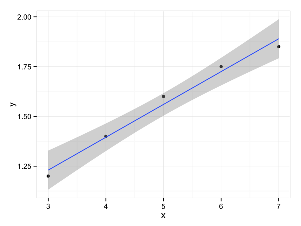
Fit the regression line:
fit<-lm(y~x,data=Q8)
fit
Call:
lm(formula = y ~ x, data = Q8)
Coefficients:
(Intercept)            x
      0.735        0.165
The equation of the regression line therefore is:
y = 0.735 + 0.165 × x
2. What is the correlation coefficient?
cor(Q8$x,Q8$y,method='pearson')
[1] 0.9913889
The correlation coefficient therefore is 99%.
3. Interpolate the y-value for x = 5.5
y(x = 5.5) = 0.735 + 0.165 × 5.5 = 1.6425
4. Extrapolate the y-values for x = 0.1 and x = 15
y(x = 0.1) = 0.735 + 0.165 × 0.1 = 0.7515
y(x = 15) = 0.735 + 0.165 × 15 = 3.21
The data is also provided in Q8-2.rda (the data frame is called Q8Extended). To call the data in the console:
Q8Extended
      x     y
1   0.1 -1.25
2   0.2 -0.70
3   1.0  0.40
4   2.0  0.90
5   3.0  1.20
6   4.0  1.40
7   5.0  1.60
8   6.0  1.75
9   7.0  1.85
10  8.0  1.95
11  9.0  2.05
12 10.0  2.10
13 12.0  2.25
14 14.0  2.35
15 15.0  2.40
5. Plot these data in a graph.
To create a scatterplot to evaluate the relation between the two variables (without a regression line):
ggplot() +
geom_point(aes(x = x,y = y),data=Q8Extended) +
theme_bw()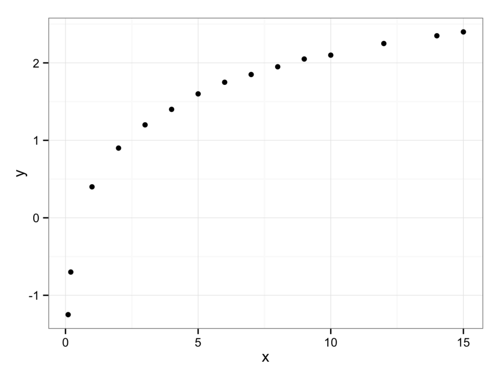
6. What is the relation between x and y and what is the value of the correlation coefficient?
A linear regression is clearly hopeless:
ggplot() +
geom_point(aes(x = x,y = y),data=Q8Extended) +
geom_smooth(aes(x = x,y = y),data=Q8Extended,method = 'lm') + theme_bw()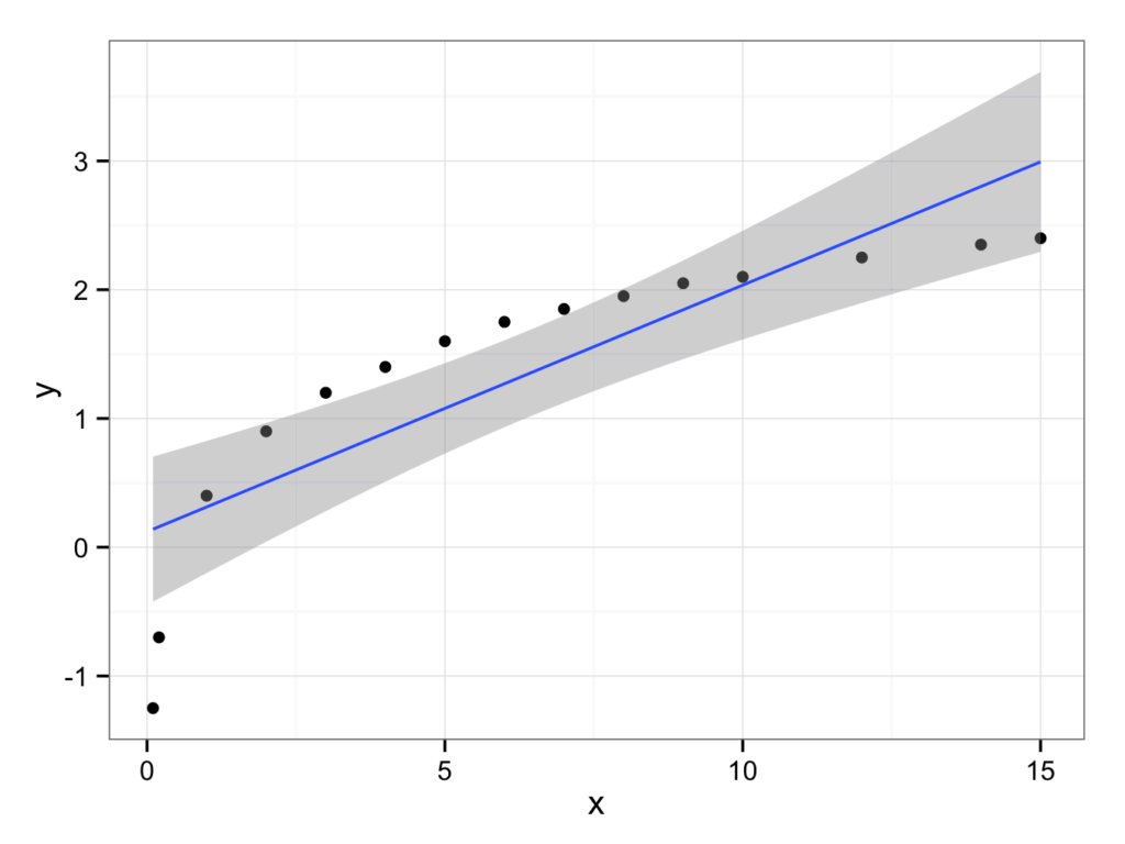
x and y appear to have a logarithmic relation and the general equation of the regression line is:
y = b + a × log(x)
or:
ggplot() +
geom_point(aes(x = log(x),y = y),data=Q8Extended) +
geom_smooth(aes(x = log(x),y = y),data=Q8Extended,method = 'lm') + theme_bw()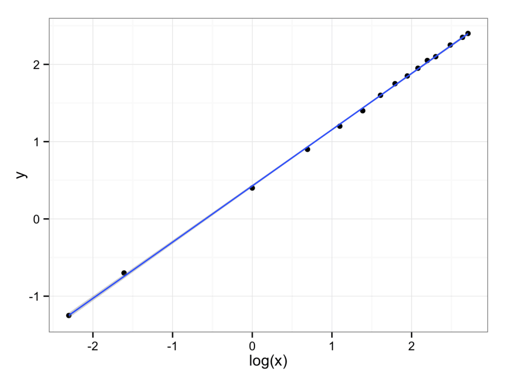
The equation of the regression line is:
fit<-lm(y~log(x),data=Q8Extended)
fit
Call:
lm(formula = y ~ log(x), data = Q8Extended)

Coefficients:
(Intercept)       log(x)
0.4271       0.7276
Or:
y = 0.4271 + 0.7276 × log(x)
Alternatively, you could plot the data on a logarithmic x axis:
ggplot(data=Q8Extended, aes(x=x, y=y)) +
geom_point() +
coord_trans(x = "log10") +
theme_bw()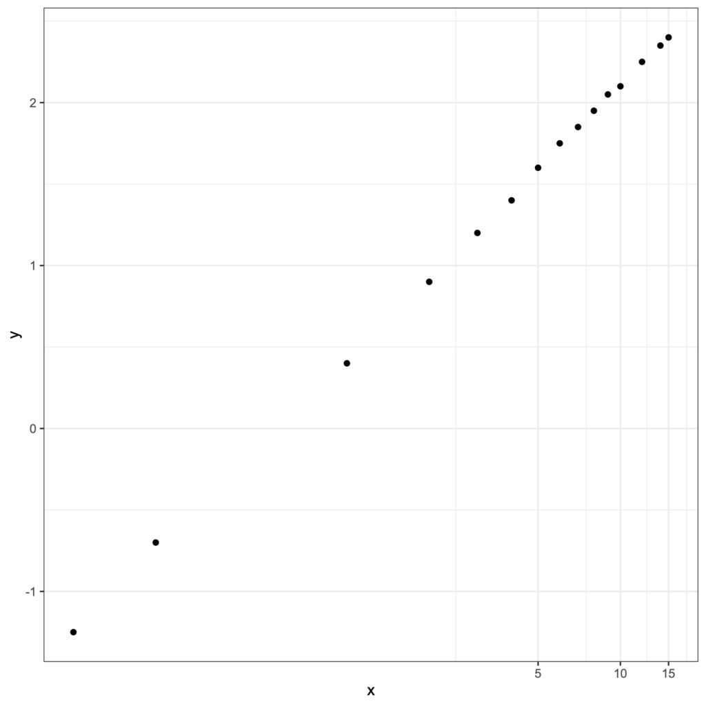
To find the value of the correlation coefficient:
cor(log(Q8Extended$x),Q8Extended$y,method='pearson')
[1] 0.9997933
7. What are the y-values for x = 0.1 and x = 15?
As described under 6, the equation of the regression line is:
y = 0.4271 + 0.7276 × log(x)
Therefore,
y(x = 0.1) = 0.4271 + 0.7276 × log(0.1) ≈ -1.25
y(x = 15) = 0.4271 + 0.7276 × log(15) ≈ 2.40
This question illustrates again the danger of extrapolating data!
8. The scatterplot and line x=y can be created with the following command in the R console:
ggplot() +
geom_point(aes(x = Lafayette,y = iPhone),data=goniometer) +
theme_bw() +
geom_abline(data=goniometer, intercept = 0.0,slope = 1.0,
  colour = '#339900', linetype = 2)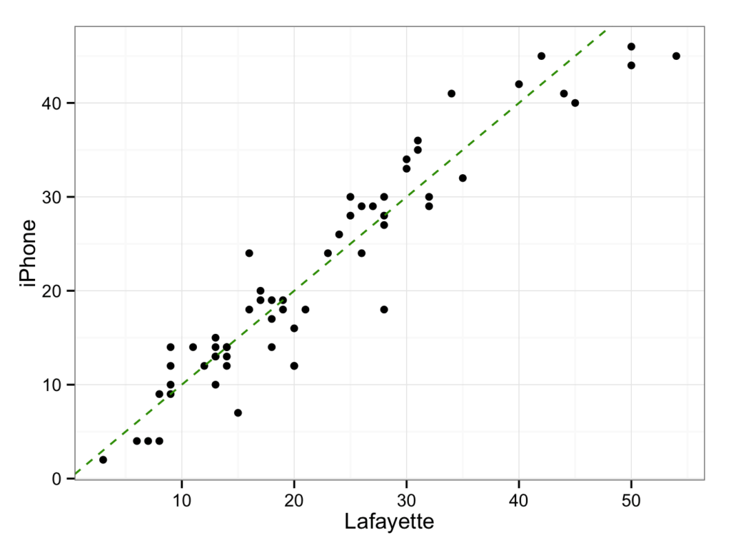
9. To calculate the Pearson correlation coefficient:
cor(goniometer$Lafayette,goniometer$iPhone,method="pearson")
[1] 0.9473263
Therefore, Pearson’s correlation coefficient is 95%.
10. To calculate the ICC:
library(irr)
icc(goniometer,model="twoway",type="agreement")
 Single Score Intraclass Correlation
   Model: twoway
   Type : agreement
   Subjects = 60
     Raters = 2
   ICC(A,1) = 0.948
 F-Test, H0: r0 = 0 ; H1: r0 > 0
 F(59,59.8) = 37 , p = 1.6e-31
 95%-Confidence Interval for ICC Population Values:
  0.914 < ICC < 0.968
Therefore, the ICC is 95%.