Box Plot

Box and whisker plots, or just box plots are used for the presentation of continuous data, that can be grouped in categories. The box represent the interquartile range and the horizontal line within it the median value. The whiskers represent the upper and lower adjacent values that lie within 1.5 times the interquartile range (although the definition may very between software programs). Any value outside the whiskers is marked separately as an ‘outlier’.

Download and open the plotbox.rda dataset for this example. The data set contains the maximum flexion in 20 patients before and after a manipulation under anaesthesia. The data can be shown by:

plotbox
   Pre Post
1   94  115
2   95  103
3   89  113
4   89  122
5  101  103
6   76   93
7  102  118
8  104  102
9  103   81
10  93  102
11 101  124
12  92  130
13  77  103
14  95  125
15  89  108
16  95  106
17  92  105
18  84   89
19  83  113
20  86   86

To create a box and whisker plot of the pre-mua data:

pre <- ggplot(data=plotbox, aes(y=Pre,x='PreMUA')) +
geom_boxplot()
pre

Add a black and white theme, a title and axes labels:

pre <- pre +
ggtitle('Preoperative flexion') +
xlab(label='Status') +
ylab(label='max flexion [deg]') +
theme_bw()
pre

To create a similar box and whisker plot of the post-mua flexion:

post <- ggplot(data=plotbox, aes(y=Post,x='PostMUA')) +
geom_boxplot() +
ggtitle('Postoperative flexion') +
xlab(label='Status') +
ylab(label='max flexion [deg]') +
theme_bw()
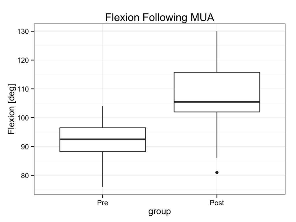
post

The preMUA plot looks symmetrical with the median in the middle of the box. However, the postMUA plot is clearly skewed as the median is located in the lower part of the box (right skewed, because the tail is to the ‘right’ or higher values). This is also reflected in the descriptive statistics:

summary(plotbox$Pre)
   Min. 1st Qu.  Median    Mean 3rd Qu.    Max. 
  76.00   88.25   92.50   92.00   96.50  104.00 
summary(plotbox$Post)
   Min. 1st Qu.  Median    Mean 3rd Qu.    Max. 
   81.0   102.0   105.5   107.0   115.8   130.0 

The mean and median are approximately the same in preMUA suggesting the data might be Normally distributed. However, postMUA this does not seem likely.

It would be nice to show both plots in one:

both <- ggplot(data=plotbox) + 
geom_boxplot(aes(y=Pre,x='Pre MUA')) +
geom_boxplot(aes(y=Post,x='Post MUA')) +
ggtitle('Flexion before and after MUA') +
xlab(label='Status') + 
ylab(label='max flexion [deg]')+
theme_bw()
both

This will show the plot with the x-axis in alphabetical order. The easiest way to change this is by regrouping the data into tidy format. Create a data-frame called ‘muapre’ for all preoperative data; the first collumn is called ‘flexion’ and the second ‘group’ (which are all “Pre”).  Similarly, a ‘muapost’ data-frame is created for all postoperative data with the same column names:

muapre<-data.frame(flexion=plotbox$Pre, group='Pre')
muapre
   flexion group
1       94   Pre
2       95   Pre
.....
.....
19      83   Pre
20      86   Pre
muapost<-data.frame(flexion=plotbox$Post, group='Post')
muapost
   flexion group
1      115  Post
2      103  Post
.....
.....
19     113  Post
20      86  Post

Now, bind the rows (rbind) together to create a new data-frame called mua:

mua<-rbind(muapre,muapost)
mua
   flexion group
1       94   Pre
2       95   Pre
.....
.....
39     113  Post
40      86  Post

Now the ‘mua’ data-frame can be used to create a grouped box and whisker plot:

muaplot <- ggplot(data=mua, aes(y = flexion, x = group)) + 
stat_boxplot() + 
ggtitle(label='Flexion Following MUA') + 
ylab(label='Flexion [deg]') +
theme_bw()
muaplot