As described, a regression line was fitted through 30 data points in the trees30.rda data set. Data were also extrapolated and it was estimated that a tree with a diameter of 500 centimetres would have a mass of 1208 kilogram. However, one should be more cautious when extrapolating data as is illustrated below. The data set has been extended and the data of 104 trees can be found in trees.rda. The data is shown by:
ExtendedTreeGirthMass
Girth Mass
1 205 251
2 213 272
3 219 335
–
–
103 522 2508
104 527 2375
The formula of the line is found by:
fit<-lm(Mass~Girth,data=ExtendedTreeGirthMass)
fit
Call:
lm(formula = Mass ~ Girth, data = ExtendedTreeGirthMass)
Coefficients:
(Intercept) Girth
-1225.413 5.874
The equation of the line therefore is:
Mass=5.874×Girth-1225.413
Please note the equation of this line is different from the one found when there were only 30 trees in the data set (Mass = 3.24×Girth -411.62).
The correlation coefficient is found by:
cor(ExtendedTreeGirthMass$Mass,ExtendedTreeGirthMass$Girth,method=’pearson’)
[1] 0.916265
A correlation coefficient of 92% does appear very satisfactory. However, if we plot the data, the fit is perhaps somewhat disappointing:
ggplot() + geom_point(aes(x = Girth,y = Mass),data=ExtendedTreeGirthMass) + theme_bw() + ggtitle(label = “Girth and Mass Trees”) + xlab(label = “Girth [cm]”) + ylab(label = “Mass [kg]”) + geom_smooth(aes(x = Girth,y = Mass),data=ExtendedTreeGirthMass,method = ‘lm’)
Code can be copied directly into the R console, but special characters like quotation marks (“) may need to be re-entered.
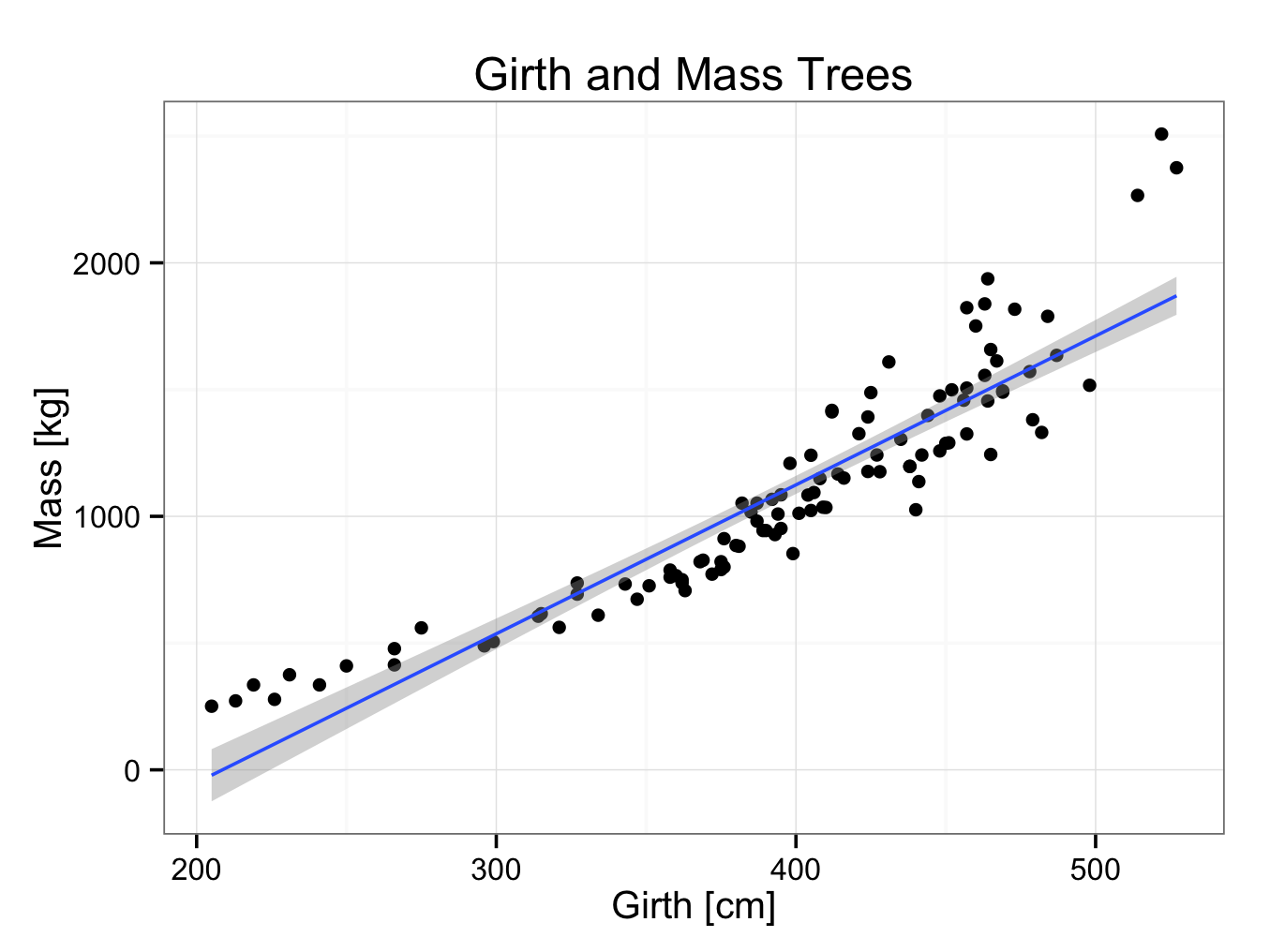 Looking at the plot, it seems an exponential relation seems more appropriate. This would also fit our understanding of growth better. This is another example why it is always advisable to plot the data and not only rely on descriptive values.
To fit an exponential regression line to the data, use the equation:
or
There are two ways to perform exponential curve fitting:
1 Transform the y axis to logarithmic scale:
ggplot() + geom_point(aes(x = Girth,y = Mass),data=ExtendedTreeGirthMass) + theme_bw() + ggtitle(label = “Girth and Mass Trees”) + xlab(label = “Girth [cm]”) + ylab(label = “Mass [kg]”) + geom_smooth(aes(x = Girth,y = Mass),data=ExtendedTreeGirthMass,method = ‘loess‘) + coord_trans(ytrans = ‘log’)
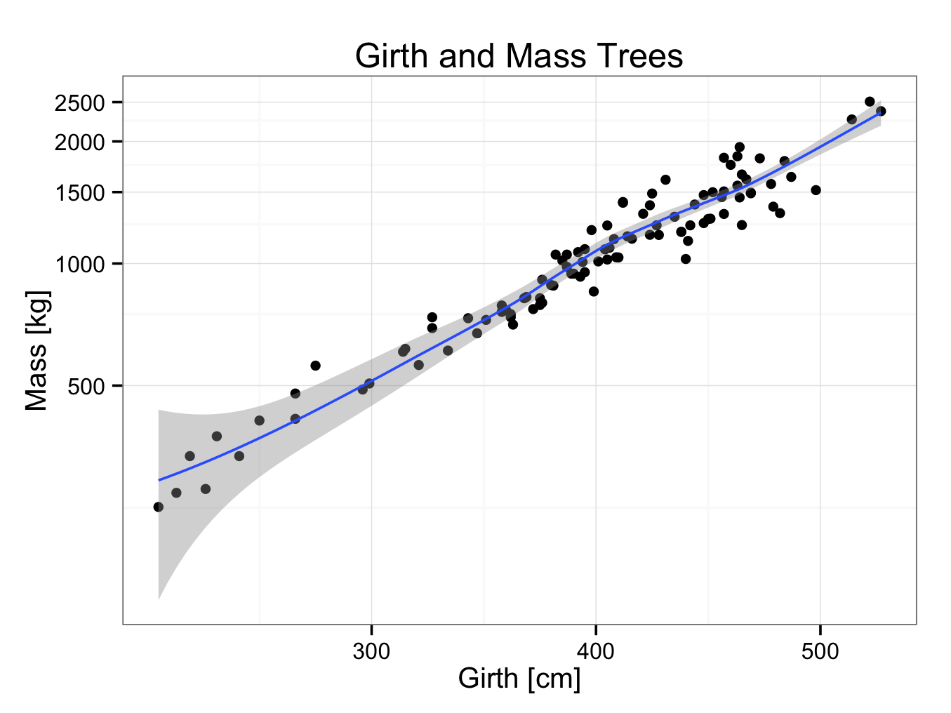 The advantage of this method is that it is very straight forward and that the original values on the axes are maintained. However, it is difficult to obtain the equation of the logarithmic regression analysis and perform inter- or extrapolation. Furthermore, the linear model gives data out of range and therefore a loess (smooth) model is required (resulting in a line that is not straight).
Please note to use loess and not lm (linear model) as method!
The code can be copied and pasted, but quotation marks (“) may need to re-entered.
2 Log tranformation:
ggplot() + geom_point(aes(x = Girth,y = log(Mass)),data=ExtendedTreeGirthMass) + theme_bw() + ggtitle(label = “Girth and Mass Trees”) + xlab(label = “Girth [cm]”) + ylab(label = “log(Mass [kg])”) + geom_smooth(aes(x = Girth,y = log(Mass)),data=ExtendedTreeGirthMass,method = ‘lm’)
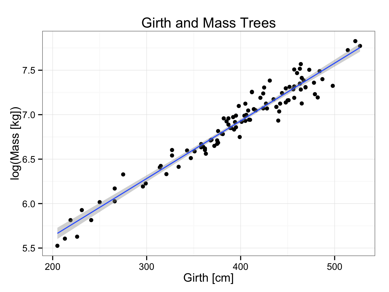
The original (untransformed) values are indicated on the x-axis, but transformed values on the y axis, making interpretation perhaps more difficult.
To find the equation of the logarithmic regression line:
fit<-lm(log(Mass)~Girth,data=ExtendedTreeGirthMass)
fit
Call:
lm(formula = log(Mass) ~ Girth, data = ExtendedTreeGirthMass)
Coefficients:
(Intercept) Girth
4.33456 0.00649
The formula of the logarithmic regression line therefore is:
Log(Mass)=0.00649×Girth+4.33456
Extrapolation with linear and log model
Using the linear model, a tree with a girth of 500 centimetres would have a mass of:
Mass=5.874×500-1225.413 ≈ 1712 kg
However, using the log model:
Log(Mass)=0.00649×500+4.33456 =7.57956
Mass ≈ 1958 kg
The prediction with the logarithmic model fits the data much better.