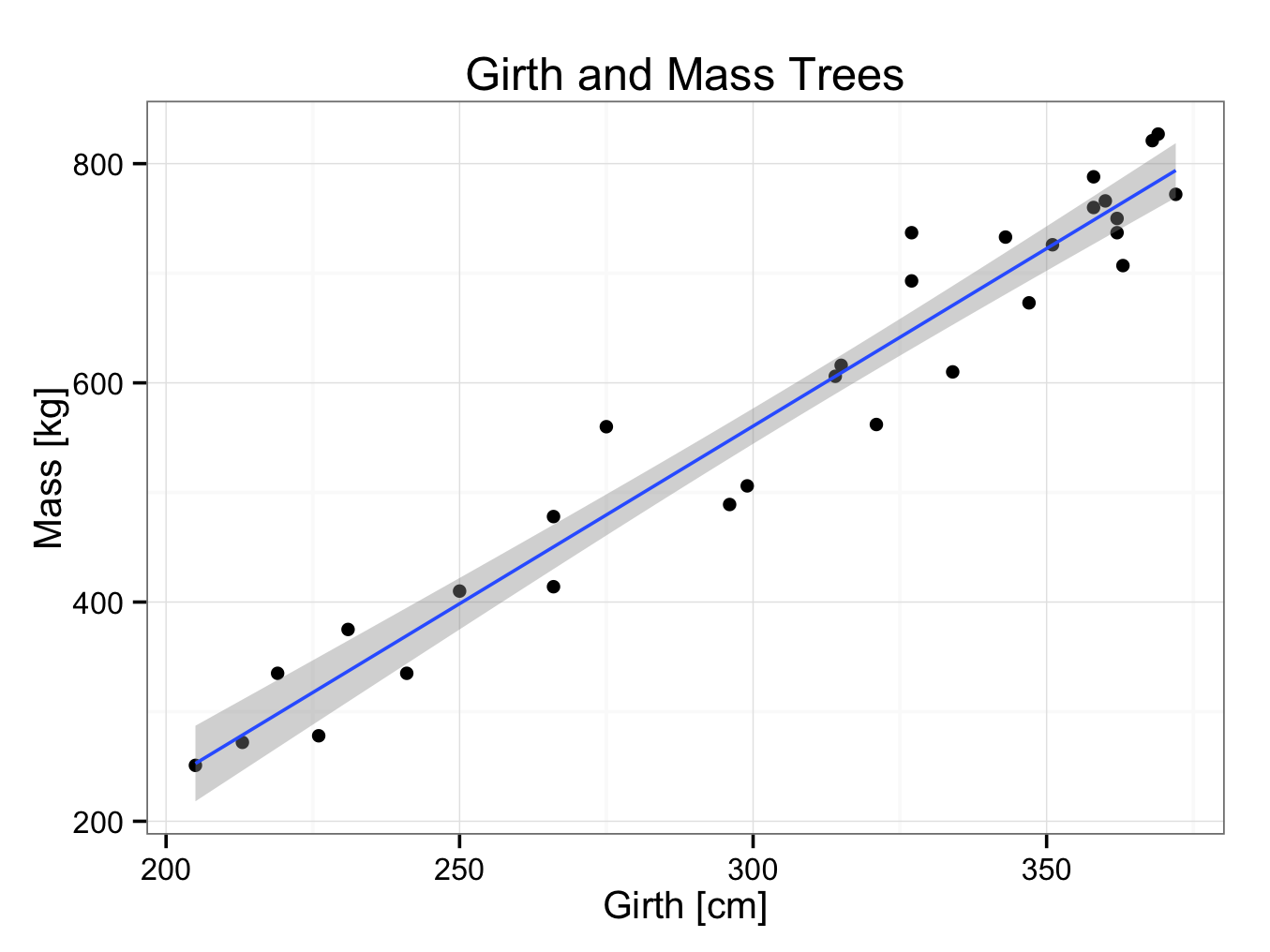
As described, a regression line was fitted through 30 data points in the trees30.rda data set.
The formula of the line is found by:
fit<-lm(Mass~Girth,data=TreeGirthMass)
fit
Call:
lm(formula = Mass ~ Girth, data = TreeGirthMass)
Coefficients:
(Intercept) Girth
-411.62 3.24
Therefore the equation of the regression line is:
Mass = 3.24×Girth -411.62
This is the equation of the line showing the relation between girth and mass of a tree. In the example, the tree had to be chopped down to measure its mass. It would be nice to estimate the mass of a tree by only measuring its girth (without chopping it down; so the profit margin could be estimated)! From the equation we can estimate the mass of a tree with a girth of 280 centimetres:
Mass = 3.24×280 -411.62 = 495.58 kg
The estimation we made is within the range we have measured. This process is called interpolation. Of course, it is also possible to let R do this directly using the predict function. The predict function takes the model (fit) as first argument and a data frame with the value(s) of the Girth:
predict(fit, data.frame(Girth = 280))
1
495.7158
The difference with the manual method above is due to rounding error.
Similarly, we can estimate the mass of a tree outside the range we have measured. This process is called extrapolation. For example, to estimate the mass of a tree with a girth of 500 cm:
Mass = 3.24×500 -411.62 = 1208.38 kg
Or in R:
predict(fit, data.frame(Girth = 500))
1
1208.622
Obviously, one has to be far more cautious with estimations found by means of extrapolation than with interpolation.
It is also possible to predict a range of value in R:
predict(fit, data.frame(Girth = c(280, 500)))
1 2
495.7158 1208.6223