One often wants to know if there is a relation or association between two variables. To look if there is such a relation, an experiment can be designed. This experiment provides us data that can be plotted (scatterplot). Next, a line or curve that best fits these data is drawn. The mathematical equation of the curve gives us the relation. Most commonly, a straight line is fitted through the data and this process is called linear curve fitting. It is however also possible to fit non-linear curves to data.
Linear Curve fitting
Linear curve fitting will be explained with an example. It is suggested, there may be a relation between the girth and mass of a tree. The girth of 30 trees and their corresponding mass was measured. The data can be found in trees30.rda. Open the data set in JGR and the data can be seen:
TreeGirthMass
Girth Mass
1 205 251
2 213 272
3 219 335
4 226 278
5 231 375
6 241 335
7 250 410
8 266 414
9 266 478
10 275 560
11 296 489
12 299 506
13 314 606
14 315 616
15 321 562
16 327 693
17 327 737
18 334 610
19 343 733
20 347 673
21 351 726
22 358 760
23 358 788
24 360 766
25 362 750
26 362 737
27 363 707
28 368 821
29 369 827
30 372 772
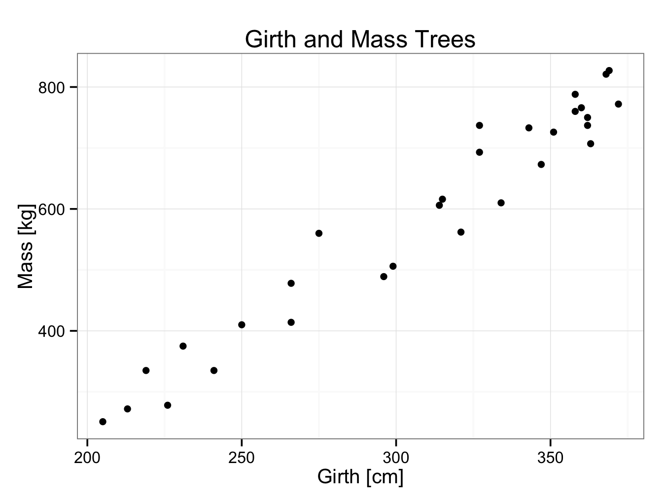
As can be seen, there are trees with a girth between 200 and 375 centimetres. In this case, the girth is the independent variable and the mass the dependent variable (if trees were selected according to their mass rather than girth, the mass would have been the independent variable and the girth the dependent variable). Next, the data is plotted in a scatterplot. Customary, the independent variable is plotted on the x-axis and the dependent variable on the y-axis:
ggplot() + geom_point(aes(x = Girth,y = Mass),data=TreeGirthMass) + theme_bw()
Or with a title and axes labels:
ggplot() + geom_point(aes(x = Girth,y = Mass),data=TreeGirthMass) + theme_bw() + ggtitle(label = ‘Girth and Mass Trees’) + xlab(label = ‘Girth [cm]’) + ylab(label = ‘Mass [kg]’)
In linear curve fitting, a straight line is drawn that fits the data points best. One way of doing this is to plot the data as shown above and draw a line through it with a ruler. When we draw the line, we will try to have as many data points above as below the line. This is certainly an acceptable method and seems to be no problem in the example above. However, the data do not always lie close to a straight line. If they would lie further apart, it would be more difficult to draw a straight line through them. Furthermore, this graphical method is not very consistent. A mathematical method is favoured as is far more consistent than a graphical method.
There are several mathematical methods described to fit a straight line through data points and full discussion of these is beyond the scope of this book. One method commonly used is the least square method. This is illustrated in the next graph:
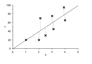 Imagine a straight line through the data points as shown. The distance of the dependent variable to this proposed line is calculated (vertical distances as indicated in the plot). Next the square of this distance is taken and all of these squares are added together. The square is taken for two reasons:
- Points below the line have a negative distance and points above the line a positive distance. They therefore tend to cancel each other out. In taking the square, all distances become positive; eliminating the problem.
- By taking the square, data points further away from the proposed line are given more ‘weight’ than those close to the line.
This process is repeated for all straight lines possible. The best fitting line is that were the sum of the squares is least. This method is therefore called the least square method. Computers are used to perform these calculations.
Regression coefficient
A straight line has the following basic equation:
y = a×x+ b
Were x is the independent variable and y the dependent variable. ‘a’ is the regression coefficient. It represents the slope of the line and can be calculated by dividing the difference in y-value to the difference in x-value at two points: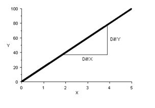 If a = 0, the line is horizontal. The larger the value of ‘a’, the more vertical (steeper) the line is:
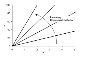 A negative value of ‘a’ corresponds to a downwards slope:
 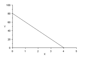 In the graph above, the regression coefficient = – 20
 .
The intercept ‘b’ is a constant for the line and represents the y-value at x = 0. If the line goes through the origin of the coordinate system (0,0), than b = 0. If the line crosses above the origin, ‘b’ is positive and if it crosses below the origin, ‘b’ is negative. In the graph above, b = 80, so:
y = -20×x +80
Returning to the example with the girths and masses of 30 trees, it is easy to add a linear regression line with a 95% confidence interval to the plot by adding the geom_smooth function to the plot (it is also possible to do this with plot builder):
ggplot() + geom_point(aes(x = Girth,y = Mass),data=TreeGirthMass) + theme_bw() + ggtitle(label = ‘Girth and Mass Trees’) + xlab(label = ‘Girth [cm]’) + ylab(label = ‘Mass [kg]’) + geom_smooth(aes(x = Girth,y = Mass),data=TreeGirthMass,method = ‘lm’)
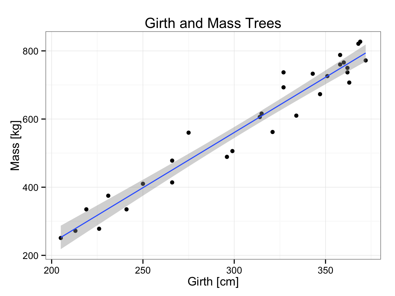 The computer has drawn the best fitting line through the data points using the least square method. In addition, the 95% confidence interval is indicated with grey shading. However, it doesn’t provide the formula of the regression line. The formula of the regression line can be found by:
fit<-lm(Mass~Girth,data=TreeGirthMass)
fit
Call:
lm(formula = Mass ~ Girth, data = TreeGirthMass)
Coefficients:
(Intercept) Girth
-411.62 3.24
The regression coefficient is 3.24 and the intercept -411.62, therefore the formula of the regression line is:
Mass = 3.24×Girth -411.62
The regression coefficient is a measure of the slope of the line. It ranges from -∞ to +∞. A regression coefficient of zero means the line is horizontal; a positive value corresponds to an upward slope and a negative value to a downward slope. The larger the value of the regression coefficient, the steeper the slope.