Parametric tests can only be used if the data are Normally distributed (or any other known distribution). Therefore, the data need to be continuous data. However, continuous data are not necessarily Normally distributed, and the data could well be skewed.
Often, we do not know how data are distributed and it is difficult to tell from our sample what the distribution of data is. The distribution could be Normal; but we are not sure. It this case we can use a statistical test to test whether the data is normally distributed or not. There are several test described to test for Normality. Examples are the Shapiro-Wilk test, Kolmogorov-Smirnov test and Quantile-Quantile plots.
If we have a large sample size (>50) we can use the Normal distribution itself and read from the graph. Usually, we perform a two sided test. This means that the alternate hypothesis could be bigger or smaller than the null hypothesis. Consequently, we have to ‘share’ the 5% between the two tail ends of the curve (2.5% at each tail end):
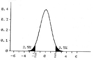
It should be noted that this is plus or minus twice the standard deviation from the mean. So, if the mean of our study group lies in each of the two dark areas on the graph; we feel this is very unlikely to be due to chance and the null hypothesis is rejected in favour of the alternate hypothesis.
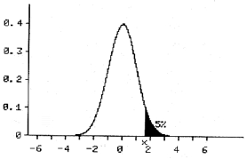
Occasionally, we know that the alternate hypothesis can only be larger than the alternate hypothesis. In that case we can use the 5% on only one tail end of the curve. This is called one sided testing.
t-Test
If the sample size is large (> 50), we can use the Normal distribution and read from graphs / tables. However, it is unusual to have such large sample sizes and often sample sizes are much smaller (around 20 to 30).Consequently, a ‘correction’ has to be made for the small sample size. This can be done using the t-test.
As example we use the skinfold.rda data on the thickness of the skinfold in patients with and without cancer. For now, let us assume we have demonstrated that the data are Normally distributed (with a test for Normality) and the t-test can be used to analyse the data. A mathematical description of the t-test is beyond the scope of this book. Suffice to say that the t-test corrects for the smaller sample size with a ‘correction factor’.
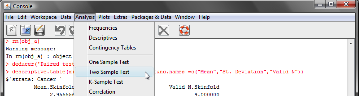
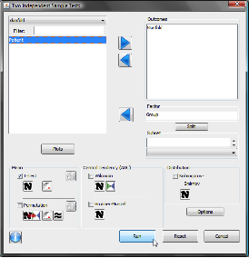
If we feed our data JGR / Deducer we can perform an unpaired t-test (a paired t-test would be before and after a treatment; so the data are paired). From the menu, select ‘Analysis‘ and ‘Two Sample Tests‘. As outcome select ‘Skinfold‘ and as Factor ‘Group‘ (nominal data). In addition to a t-test, other tests can be selected (ie non parametric Wilcoxon) as well as a Kolmogorov-Smirnov test for Normality.
Alternatively, enter in the console:
t.test(Skinfold~Group,data=skinfold)
Welch Two Sample t-test
data: Skinfold by Group
t = -2.7653, df = 26.968, p-value = 0.01013
alternative hypothesis: true difference in means is not equal to 0
95 percent confidence interval:
-3.0475746 -0.4513143
sample estimates:
mean in group Cancer mean in group No Cancer
2.955556 4.705000
or:
two.sample.test(formula=d(Skinfold) ~ Group,data=skinfold,test=t.test,alternative=”two.sided”)
Welch Two Sample t-test
mean of Cancer mean of No Cancer Difference 95% CI Lower 95% CI Upper t df p-value
Skinfold 2.955556 4.705 -1.749444 -3.047575 -0.4513143 -2.765335 26.96762 0.010134
HA: two.sided
H0: difference in means = 0
The computer calculates the p Value using the t-test:
p = 1.01 % < 5%
Therefore, the probability that the difference is due to chance is very small and the difference is statistically significant. We can therefore reject the null hypothesis in favour of the alternate hypothesis. So we conclude that there is a difference in skin fold thickness in patients with cancer and that their nutrition is poorer.
In the example above, the t-test was performed on unpaired data. A t-test can also be performed on paired samples; before and after an intervention or treatment. If the data are dependent / related, use a paired t-test. Otherwise, use an unpaired t-test.
An example of dependent data is the range of movement in the knee before and after a total knee replacement. We have two groups of data: range of movement before and after total knee replacement. The two groups are dependent and provided the data in Normally distributed; we can use the paired t-test.
On the basis of this t-test, we would reject the null hypothesis (there is no difference in skinfold thickness between cancer and non cancer patients) and we would conclude that there is a difference in skin thickness and therefore nutritional status. However, we may not have been correct in using a t-test, as we have not demonstrated Normality. We can check normality of all the skinfold thickness data:
shapiro.test(skinfold$Skinfold)
Shapiro-Wilk normality test
data: skinfold$Skinfold
W = 0.8519, p-value = 0.0008328
Please not the capital S in the Skinfold variable in the skinfold data frame (with lower case s).
The p-value is significant, suggesting the data are not Normally distributed. However, this takes both groups (Cancer and Non Cancer) together. But we have just demonstrated there is a statistical difference between the two groups and they are not likely to belong to the same distribution (p<0.05)! So, it is probably better to test for Normality in both groups separately:
shapiro.test(skinfold$Skinfold[which(skinfold$Group ==’No Cancer’)])
Shapiro-Wilk normality test
data: skinfold$Skinfold[which(skinfold$Group == “No Cancer”)]
W = 0.8856, p-value = 0.0223
and
shapiro.test(skinfold$Skinfold[which(skinfold$Group ==’Cancer’)])
Shapiro-Wilk normality test
data: skinfold$Skinfold[which(skinfold$Group == “Cancer”)]
W = 0.8047, p-value = 0.02309
The [which(skinfold$Group ==’No Cancer’)] part only selects the ‘No Cancer’ patients from the data frame.
In addition, quantile-quantile plots could be help:
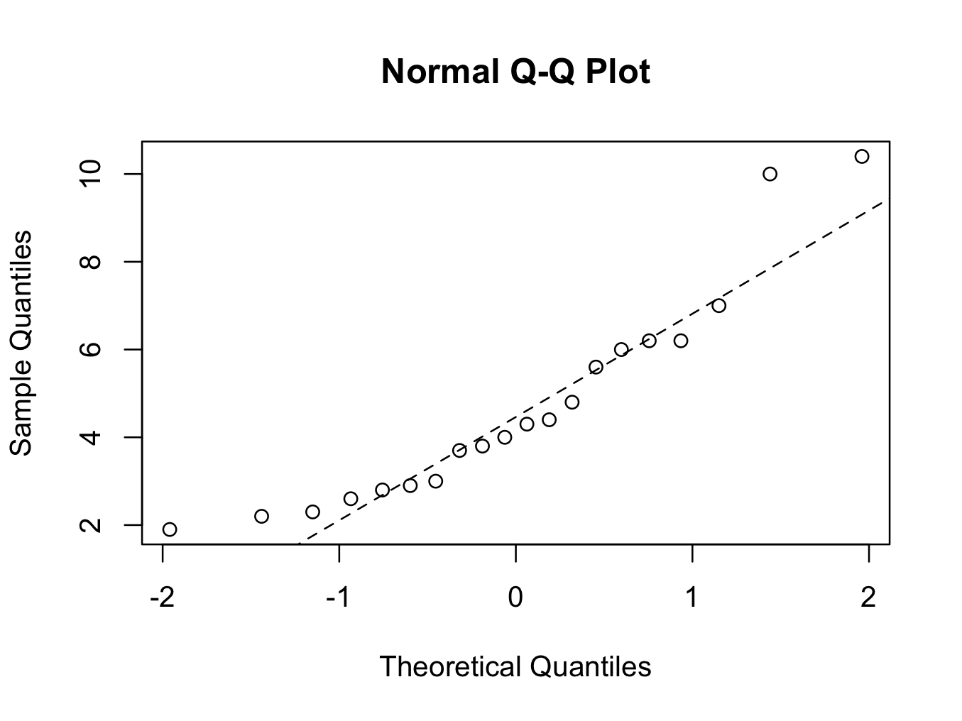
For the ‘No Cancer’ group:
qqnorm(skinfold$Skinfold[which(skinfold$Group ==’No Cancer’)])
qqline(skinfold$Skinfold[which(skinfold$Group ==’No Cancer’)],lty=2)
 and for the ‘Cancer’ group:
qqnorm(skinfold$Skinfold[which(skinfold$Group ==’Cancer’)])
qqline(skinfold$Skinfold[which(skinfold$Group ==’Cancer’)],lty=2)
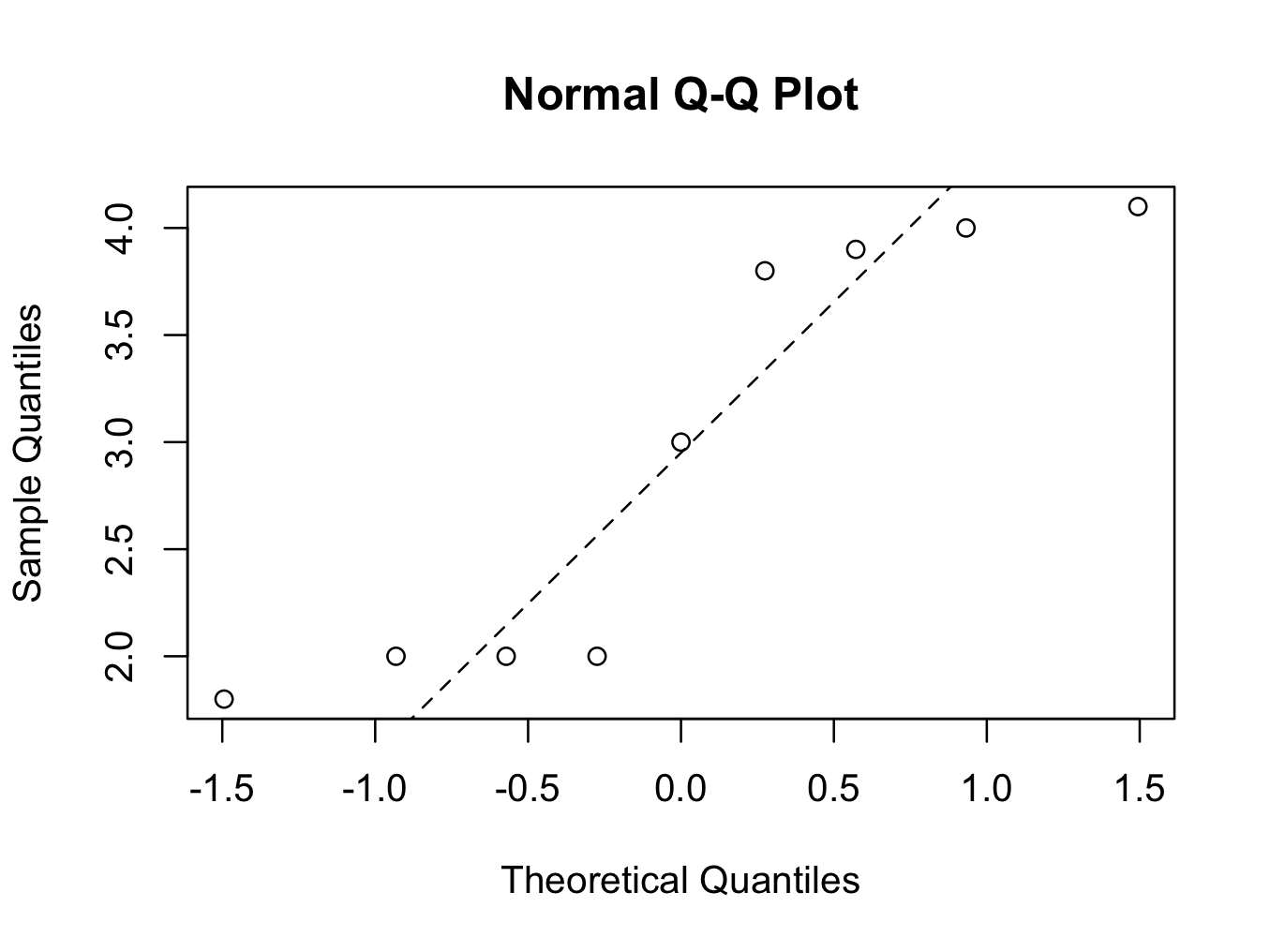 The number of patients in the ‘Cancer’ group is very small (9), but both groups fail the Normality tests. It is therefore more appropriate to use a non parametric test, in which Normality is not a requirement.