If data are not Normally distributed, a non parametric test should be used.
There are many non parametric tests described, and it is impossible to name / lists them all. We will discuss three tests; using the example data in skinfold.rda.
- Sign test
- Chi Square test
- Fisher Exact test
- Mann-Whitney U test / Wilcoxon test
It has been shown that the data are not Normally distributed. Therefore, we can not use parametric statistics and will have to use non parametric tests instead. The skinfold data will be analysed with each of the four tests mentioned above.
Sign Test
This is the most basic type of non parametric test. As the name implies, it uses the plus or minus sign to differentiate. The data is transformed; if the skin fold is smaller or equal to 4 mm, we indicate this by a minus sign and if the skin fold is greater than 4 mm by a plus sign. The data can than be summarised in a contingency table (row: skin thickness, column: cancer or not):
| No Cancer | Cancer | Total | |
|---|---|---|---|
| Total | 20 | 9 | 29 |
| <= 4 mm | 10 | 8 | 18 |
| > 4 mm | 10 | 1 | 11 |
Therefore, of the patients with cancer, there is only 1 out of 9 patients who has a skin thickness of more than 4 mm; whilst 50% of the patients without cancer had a skin fold thickness of more than 4 mm. Is this due to chance or is there a statistically significant difference?
The probability of plus is 50% and the probability of minus is 50%.
If we test two sided we need to calculate the probability that:
P = 0 out of 9 patients > 4 mm + 1 out of 9 patients > 4 mm
8 out of 9 patients < 4 mm + 9 out of 9 patients < 4 mm
So:
P < 5%, therefore statistically significant.
It is straight forward to perform a binomial test in the JGR / R console:
binom.test(1,9)
Exact binomial test
data: 1 and 9
number of successes = 1, number of trials = 9, p-value = 0.03906
alternative hypothesis: true probability of success is not equal to 0.5
95 percent confidence interval:
0.002809137 0.482496515
sample estimates:
probability of success
0.1111111
Therefore, the null hypothesis is rejected in favour of the alternate hypothesis and it is concluded that there is a difference in skin thickness between cancer patients and other patients.
Chi Square Test (χ^2 test)
Instead of the sign test, the Chi Square test can be used. There are prerequisites for the Chi Square test. These are:
- Random sample
- Sufficient sample size
- Independence of the observations
- Expected cell count at least 5 in 2 by 2 tables or at least 5 in 80% of larger tables, but no cells with an expected count of 0.
For now, lets assume the prerequisites have been met. Again, we look at the table (these are the observed frequencies):
| No Cancer | Cancer | Total | |
|---|---|---|---|
| Total | 20 | 9 | 29 |
| <= 4 mm | 10 | 8 | 18 |
| > 4 mm | 10 | 1 | 11 |
In total, there are 18 out of 29 patients with a skin fold thickness of <= 4 mm. If there were no difference between the two groups, we would expect 20 × 18 / 29 patients in the ‘No Cancer’ Group and 9 × 18 / 29 patient in the ‘Cancer’ group with a skin thickness <= 4 mm. These are called the expected frequencies. Similarly, we would expect 20 × 11 / 29 patients in the ‘No Cancer’ group and 9 × 11 / 29 patients in the ‘Cancer group with a skin thickness > 4 mm. Or summarised in a table:
| No Cancer Observed | No Cancer Expected | Cancer Observed | Cancer Expected | Total | |
|---|---|---|---|---|---|
| Total | 20 | 20 | 9 | 9 | 29 |
| <= 4 mm | 10 | 12.4 | 8 | 5.6 | 18 |
| > 4 mm | 10 | 7.6 | 1 | 3.4 | 11 |
please note one of the expected frequencies is below 5!
Next, the Chi Square test statistic is calculated:
Where O is the observed frequency and E the expected frequency.
So:
Next we need to determine the degrees of freedom: In the observed frequencies table, there are two columns (c = 2) and two rows (r = 2). So there are (r – 1)×(c – 1) = 1 degree of freedom.
We can now look in a Chi Square distribution table (statistical table):
| Degrees of Freedom | 10% | 5% | 1% |
|---|---|---|---|
| 1 | 2.71 | 3.84 | 6.63 |
| 2 | 4.61 | 5.99 | 9.21 |
| 3 | 6.25 | 7.81 | 11.34 |
| 4 | 7.78 | 9.49 | 13.28 |
| 5 | 9.24 | 11.07 | 15.09 |
| 10 | 15.99 | 18.31 | 23.21 |
Looking in the first row under one degree of freedom:
P = 3.84 at 5% and 6.63 at 1%.
3.987093154 > 3.84 and therefore the null hypothesis can be rejected in favour of the alternate hypothesis (p < 5%).
Please note that statistical significance is demonstrated at p <= 5%, but not at p <= 1%.
In the JGR / R console:
If the 2 by 2 table has already been constructed, it is easy to perform a Chi Square test. First create a matrix that contains the data in 2 rows:
skindata<-matrix(c(10,10,8,1),nrow=2)
To show the data, call the data frame:
skindata
[,1] [,2]
[1,] 10 8
[2,] 10 1
Next, do a Chi Square test:
chisq.test(skindata,correct=FALSE)
Pearson’s Chi-squared test
data: skindata
X-squared = 3.9871, df = 1, p-value = 0.04585
Warning message:
In chisq.test(skindata, correct = FALSE) :
Chi-squared approximation may be incorrect
The ‘correct=FALSE’ option switches OFF the continuity correction (Yates) when computing the test statistic. In this case, it would be better to use the continuity correction (see below under Deducer method)!
Obviously, the result is the same as with the manual method. Again, we reject the null hypothesis in favour of the alternate hypothesis: The skin thickness is less in patients with cancer than in other patients.
To show the expected frequencies:
chisq.test(skindata,correct=FALSE)$expected
[,1] [,2]
[1,] 12.413793 5.586207
[2,] 7.586207 3.413793
Warning message:
In chisq.test(skindata, correct = FALSE) :
Chi-squared approximation may be incorrect
Please note that the prerequisites of the Chi Square test have not been met! One of the expected frequencies is less than 5, hence the warning (see below).
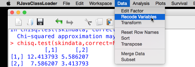
In Deducer:
Deducer can do some of the ‘leg work’ and create the 2 by 2 table directly from the data by asking it to recode a variable. This process assigns a given value (usually a 0 and 1, but other values are possible) to a new variable based on whether the source satisfies certain criteria. In this example a new variable should be coded as ‘1’ if the value of Skinfold is greater than 4, otherwise it should be ‘0’.
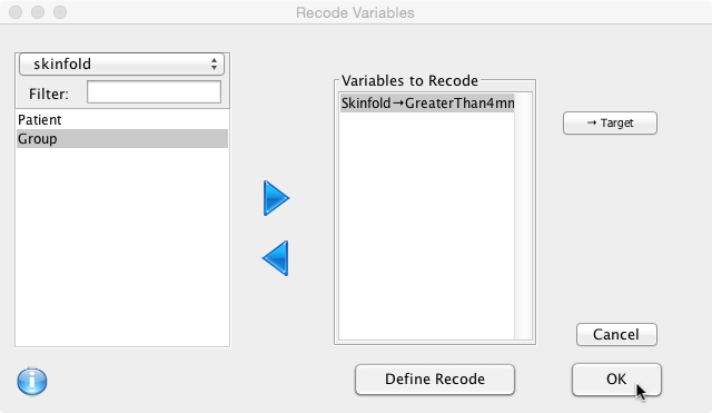
The variable ‘Skinfold’ will be recoded in a new variable called ‘GreaterThan4mm’. From the Deducer menu, choose ‘Recode Variables':
Drag Skinfold across to the ‘Variables to Recode’ box and make sure it is selected. Next, click on the ‘Target’ button.
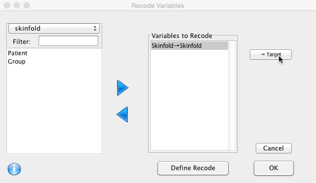
Call the new variable ‘GreaterThan4mm':

The variable Skinfold should now be mapped to the new variable:
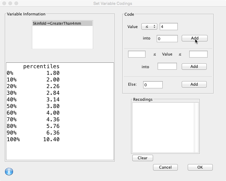
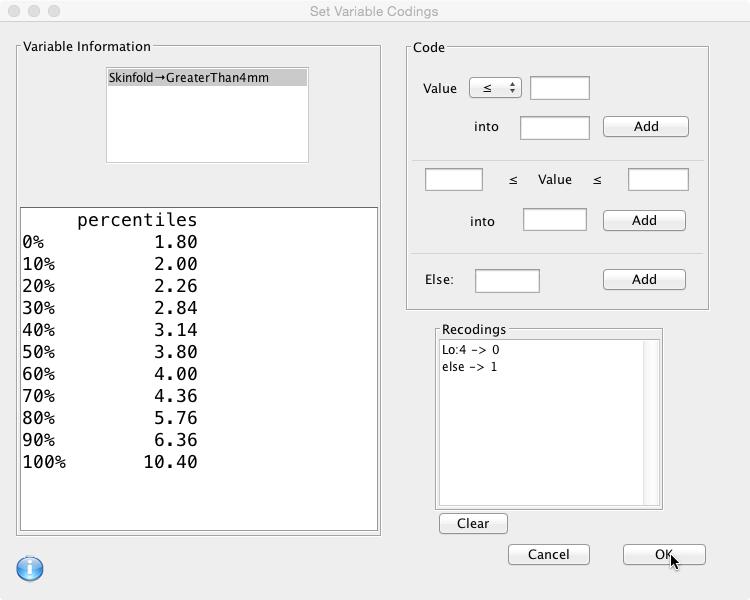
 Next click on ‘Define Recode’ to specify the rules:
- If the value of ‘Skinfold’ is less than or equal to 4, the value of ‘GreaterThan4mm’ will be 0.
- Otherwise (Else) the value will be 1.
The ‘Code box’ on the right hand side is where this is specified. First choose an operator from the drop down box, add the value and the result, then click ‘Add': Then define the second rule… and click ‘Add':
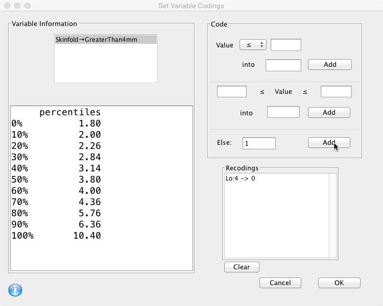
 Click ‘OK’ and ‘OK’ again:
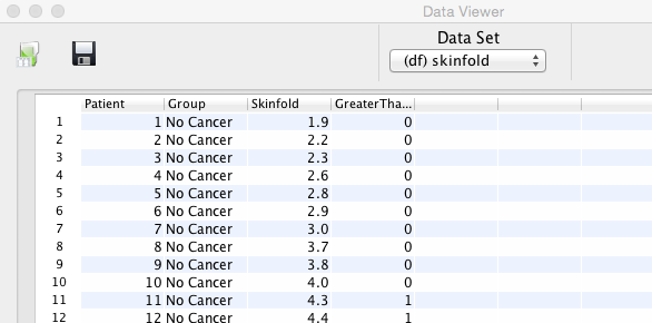
The new variable should now be available in the Data Viewer:
The ‘GreaterThan4mm’ variable can now be used to perform the Chi Square test by selecting ‘Analysis’ and then ‘Contingency Tables':

Select the variables (‘GreaterThan4mm’ as row and ‘Group’ as column):

Click on ‘Statistics’, select ‘Chi Squared’ and click OK:

Please note, the Fisher exact test has also been selected here (see below).
Different options for the Chi-Square test can be set by clicking on the cog-wheel next to the test name.
Click ‘Run’ (without altering the default options) should give the following output:
========== Table: GreaterThan4mm by Group ==========
| Group
GreaterThan4mm | Cancer | No Cancer | Row Total |
———————–| ———–| ———–| ———–|
0 Count | 8 | 10 | 18 |
Row % | 44.444% | 55.556% | 62.069% |
Column % | 88.889% | 50.000% | |
———————–| ———–| ———–| ———–|
1 Count | 1 | 10 | 11 |
Row % | 9.091% | 90.909% | 37.931% |
Column % | 11.111% | 50.000% | |
———————–| ———–| ———–| ———–|
Column Total | 9 | 20 | 29 |
Column % | 31.034% | 68.966% | |
Large Sample | Exact
Test Statistic DF p-value | Statistic DF p-value
Chi Squared 2.506 1 0.113 |
Fishers Exact | 0.096
Please note that the Test Statistic (2.506) is different than that with the console method. This is because Deducer switches ON (Correct = TRUE) the continuity correction (Yates) when computing the test statistic: One half is subtracted from all |O-E| differences; however, the correction will not be bigger than the differences themselves.
The Yates continuity correction is used for 2 by 2 tables to prevent overestimation with small data (as here). This is because the Chi Square distribution is continuous and the 2 by 2 table is dichotomous (not continuous). It is recommended that, if the expected frequencies are below 10, Yates continuity correction is used.
As a consequence of using the Yates’ continuity correction, the test becomes non significant!
To obtain the same result in the console:
chisq.test(skindata,correct=TRUE)
Using this method, the null hypothesis can’t be rejected and it is concluded there is no difference in the skin thickness between cancer patients and other patients. As one of the expected frequencies is below 5, it is perhaps more appropriate to use a Fisher Exact test.
Fisher Exact test
The output in the Chi Square test gives a warning that the approximation may be incorrect. This is because not all prerequisites for the Chi Square test have been met. One of the cells has an expected frequency of less than 5 (3.413); therefore the Chi Square test may be incorrect and a Fisher Exact test is more appropriate. To perform a Fisher Exact test:
fisher.test(skindata)
Fisher’s Exact Test for Count Data
data: skindata
p-value = 0.0959
alternative hypothesis: true odds ratio is not equal to 1
95 percent confidence interval:
0.002571797 1.319280078
sample estimates:
odds ratio
0.1333924
The Fisher Exact test, does not reject the null hypothesis as the p-value is 0.0959.
The Fisher exact test can also be performed by selecting the appropriate option box in the Deducer dialogue (see above).
Mann-Whitney U Test / Wilcoxon Test
This test has several names: Mann–Whitney U test, Mann-Whitney-Wilcoxon test, Wilcoxon rank sum test, Wilcoxon-Mann-Whitney test. It is a non parametric test for two independent samples of continuous data. It is very similar to the t-test, but the data does not have to be Normally distributed. There doesn’t seem to be agreement in the literature regarding the nomenclature of this test. In this book, we will use the name Wilcoxon test (as used in the R programming language).
We continue with the same example (skinfolds).
It has been demonstrated that it was not appropriate to use the t-test as the data are not Normally distributed. Subsequently, the data were transformed and a Chi Square test was performed. The Chi Square test without continuity correction rejected the null hypothesis. However, not all prerequisites were met and its use probably inappropriate. The Chi Square test with Yates’ continuity correction (should be used if expected frequencies are below 10) and the Fisher Exact test were both insignificant. What about the Wilcoxon test?
The Wilcoxon test is performed on continuous data, but Normality is not a requirement. The test is more powerful than the Sign and Chi Square test, but less versatile. In the previous sections, the Sign and Chi Square test were used after transforming the data. However, it is unnecessary to transform the data to nominal data and normally the most powerful test available is used within its operational conditions. The Wilcoxon test is the most appropriate test to use for the skinfold data.
In the JGR / R console:
Either:
wilcox.test(skinfold$Skinfold~skinfold$Group,correct=FALSE)
Wilcoxon rank sum test
data: skinfold$Skinfold by skinfold$Group
W = 46.5, p-value = 0.04011
alternative hypothesis: true location shift is not equal to 0
Warning message:
In wilcox.test.default(x = c(1.8, 2, 2, 2, 3, 3.8, 3.9, 4, 4.1), :
cannot compute exact p-value with ties
or:
wilcox.test(Skinfold~Group,data=skinfold,correct=FALSE)
gives the same result.
As the data are continuous, the ‘correct=FALSE’ option is selected so that no continuity correction is used in the calculation of the p-value.
The p=value is significant and therefore the null hypothesis is rejected in favour of the alternative hypothesis and it is concluded that there is a difference in the skin thickness of cancer patients and other patients.
In Deducer / JGR:
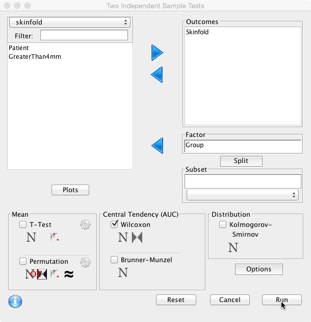
Very similar to performing a t-test as described. Select ‘Analysis’, ‘Two Sample Test’, tick ‘Wilcoxon’ and click ‘Run':
gives the same result as above.