Bland-Altman plots 1 are used to display agreement between two investigations / tests in terms of repeatability and reproducibility. If one of the measures is a gold standard, the plot can be used to display bias of the alternative test. Download the plotba.rda dataset for this example.
The data set contains measurements of two ways of measuring the haemoglobin concentration, a non-invasive way and the ‘gold standard’ laboratory test. The measurements are in g / L.
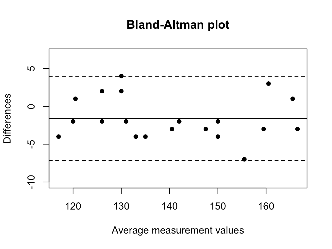
The Bland-Altman function can be used to create the plot. Copy the code to the clipboard, paste it into the console and hit return. The function is now available in R.
baplot <- function(m1, m2, ...) {
# m1 and m2 are the measurements and the input arguments of the funtion
	means <- (m1 + m2) / 2
	diffs <- m1 - m2
	mdiff <- mean(diffs)
	sddiff <- sd(diffs)
	# Compute the figure limits
	ylimh <- mdiff + 3 * sddiff
	yliml <- mdiff - 3 * sddiff
	# Plot data
	plot(diffs ~ means, xlab = "Average measurement values",pch=16,
	ylab = "Differences", ylim = c(yliml, ylimh), ...)
	abline(h = mdiff) # Center line
	# Standard deviations lines
	abline(h = mdiff + 1.96 * sddiff, lty = 2)
	abline(h = mdiff - 1.96 * sddiff, lty = 2)
	title("Bland-Altman plot")
}
The function can be called by entering baplot(variable1, variable2). In the plotba data frame, the variables are: noninvasive and lab. Therefore, the plot can be created by:
baplot(plotba$noninvasive, plotba$lab)
 To obtain the mean measurement values:
mean(plotba$noninvasive)
[1] 139.5
mean(plotba$lab)
[1] 141.1
Therefore, the non-invasive method underestimates the haemoglobin concentration as compared to the gold standard. This can also be seen in the plot, as the mean difference is below zero (solid horizontal line) and the non-invasive method is biased as compared to the gold standard; underestimating its value.
A wide range (large difference between the dotted horizontal lines) indicates poor agreement between readings.
When interpreting Bland-Altman plots, it is also important to look at patterns in the diagram. It may be that the agreement varies according to the magnitude of the measurement.
Plot axes labels can be altered by editing the baplot function.
More versatile plots can be created with the ggplot2 library 2:
Again, download the plotba.rda dataset for this example. Calculate the mean of the two observations and the difference between the two observations:
> head(plotba)
number noninvasive lab
1 1 131 135
2 2 125 127
3 3 132 128
4 4 146 149
5 5 148 152
6 6 115 119
# calculated the mean between the two methods:
plotba$means <- (plotba$noninvasive + plotba$lab) / 2
# calculate the difference between the two methods
plotba$diffs <- plotba$noninvasive – plotba$lab
head(plotba)
number noninvasive lab means diffs
1 1 131 135 133.0 -4
2 2 125 127 126.0 -2
3 3 132 128 130.0 4
4 4 146 149 147.5 -3
5 5 148 152 150.0 -4
6 6 115 119 117.0 -4
Calculate the mean and standard deviation of the differences:
mdiff <- mean(plotba$diffs)
sddiff <- sd(plotba$diffs)
mdiff
[1] -1.6
sddiff
[1] 2.835861
Load the ggplot2 library and plot the data:
library(ggplot2)
ggplot(plotba, aes(x = means, y = diffs)) +
geom_point() +
geom_hline(yintercept = mdiff – 1.96*sddiff, colour = “blue”, linetype = 3) +
geom_hline(yintercept = mdiff + 1.96*sddiff, colour = “blue”, linetype = 3) +
geom_hline(yintercept = mdiff, colour = “black”, linetype = 2) +
theme_bw(base_size= 16) +
ggtitle(“Bland-Altman plot”) +
scale_y_continuous(“Differences”, limit = c(mdiff – 3*sddiff, mdiff + 3*sddiff)) +
scale_x_continuous(“Average Measurement Values”)
