Histograms, look a bit like bar charts but are fundamentally different. The ‘bars’ or bins touch each other to indicate the data are continuous and not categorical. The bin size can be altered and it is important to select an appropriate bin size for the data. This is illustrated in the example below.
Download the heights.rda dataset for this example. This data-set contains the heights of 2000 heights, 1000 belonging to Group1 (female) and 1000 belonging to Group1 (male). It is easy to obtain some descriptive statistics:
descriptive.table(vars = d(Group1,Group2),data= heights,
+ func.names =c(“Valid N”,”Mean”,”Median”,”St. Deviation”,”Minimum”,”Maximum”))
$`strata: all cases `
Valid N Mean Median St. Deviation Minimum Maximum
Group1 1000 164.9281 164.9158 4.888238 147.5271 179.0782
Group2 1000 178.5239 178.6976 15.284486 125.4151 232.9516
In each group, the mean and median are very similar. This suggests the distribution may well be Normal. The standard deviation of Group2 is considerably larger than that of Group1, indicating the data are more dispersed in Group2.
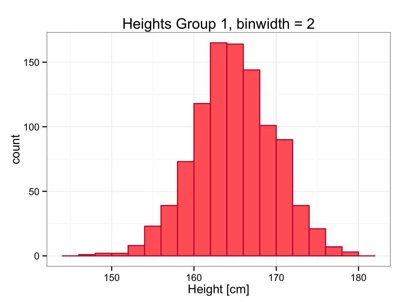
To create a histogram of Group1:
ggplot() + geom_bar(aes(y = ..count..,x = Group1),data=heights,colour = ‘#cc0033′,fill = ‘#ff6666′,binwidth = 2.0) +
ggtitle(label = ‘Heights Group 1′) +
xlab(label = ‘Height [cm]’) +
theme_bw()
If you are using ggplot < 0.9.2, the title can be set using: opts(title=’Heights Group 1′)
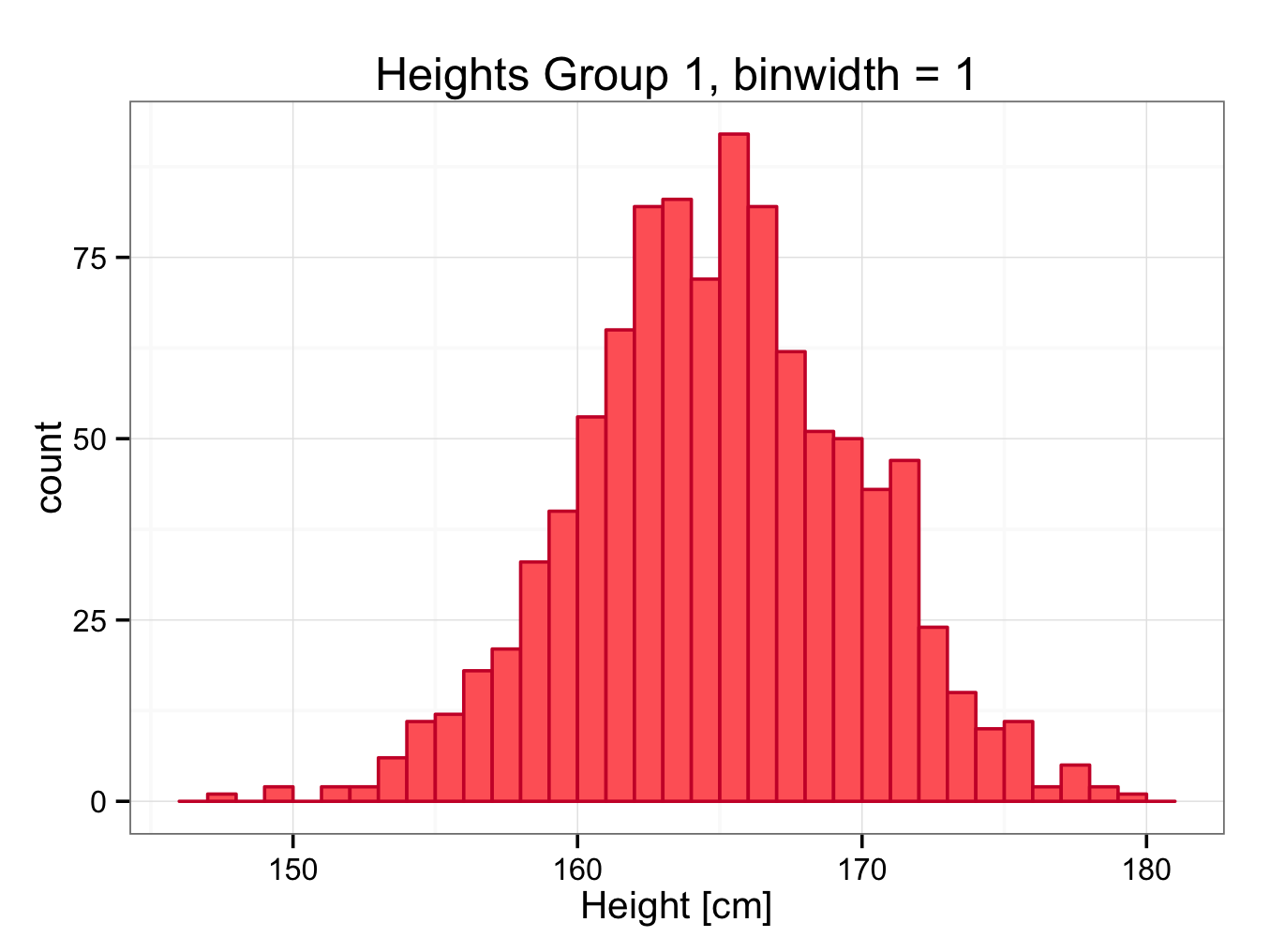
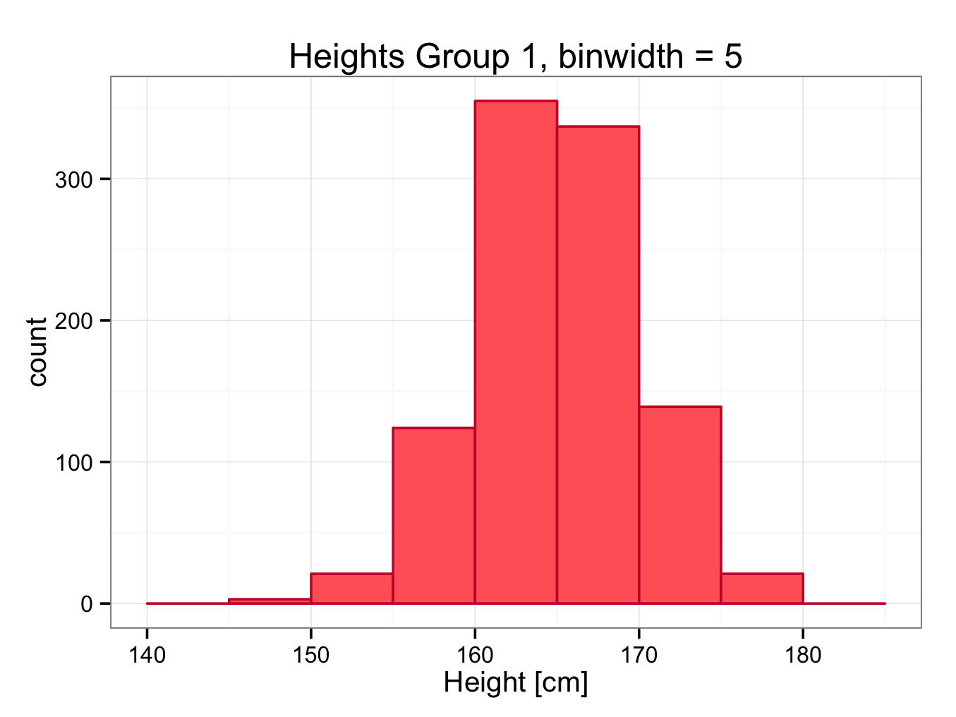
A bin width of 2.0 seems appropriate here as is illustrated in the plots below with bin width set at 1.0, 2.0 and 5.0 respectively:
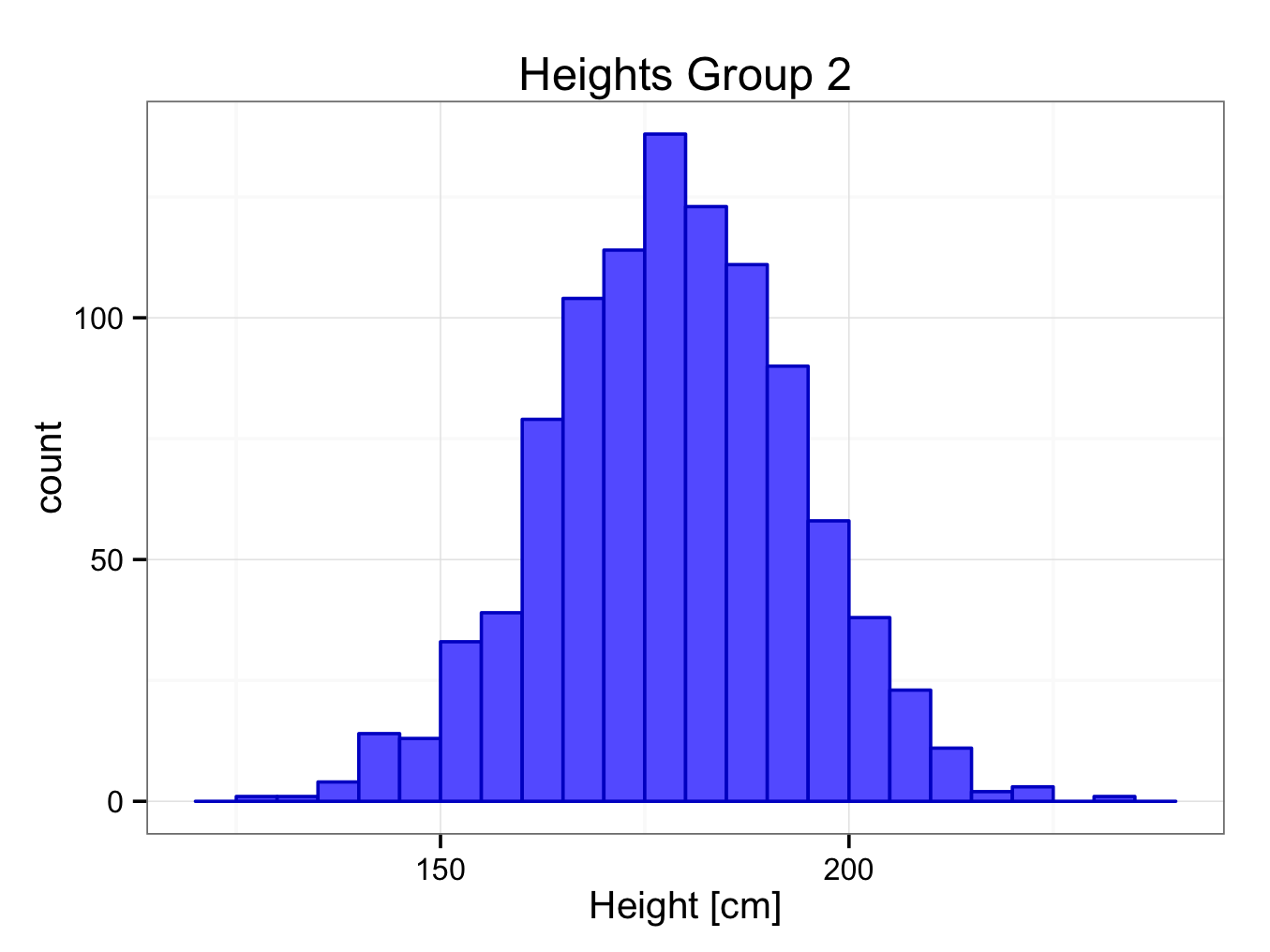
 Similarly, a histogram of Group2 (5.0 is a more appropriate bin width here than 2.0):
ggplot() +
geom_bar(aes(x = Group2),data=heights,colour = ‘#0000cc’,fill = ‘#6666ff’,binwidth=5.0) +
ggtitle(label = ‘Heights Group 2′) +
xlab(label = ‘Height [cm]’) +
theme_bw()
If you are using ggplot < 0.9.2, the title can be set using: opts(title=’Heights Group 2′)
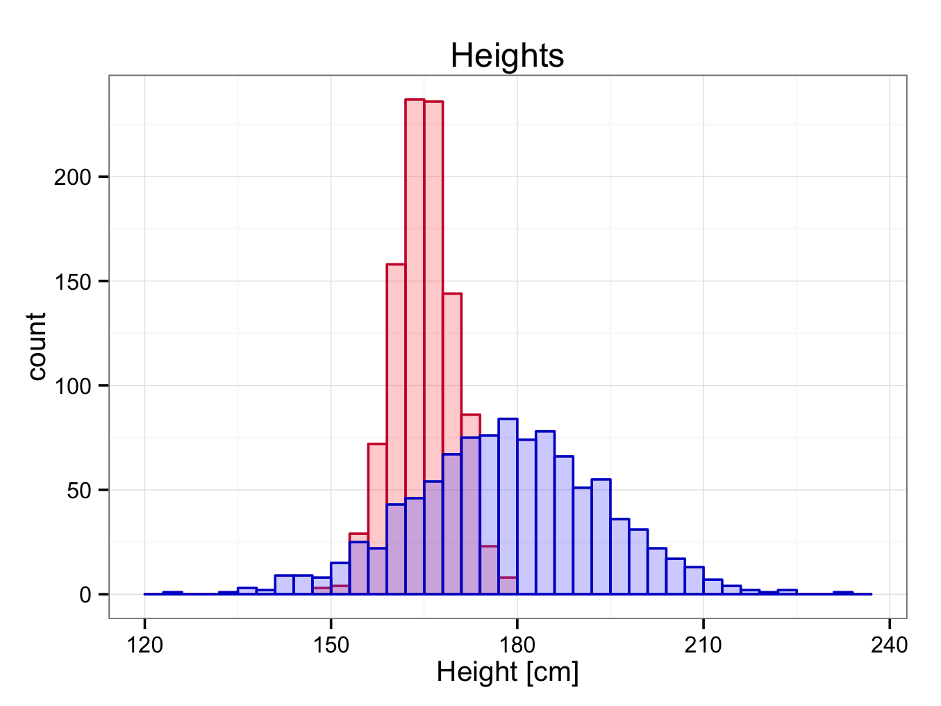
 To show both histograms in one plot, both histograms should have the same bin width (here 3.0 as a compromise). In addition, transparency has been introduced to make both histograms visible through each other (alpha=0.3):
ggplot() +
geom_bar(aes(y = ..count..,x = Group1),data=heights,colour = ‘#cc0033′,fill = ‘#ff6666′,alpha = 0.3, binwidth = 3.0) +
geom_bar(aes(y = ..count..,x = Group2),data=heights,colour = ‘#0000cc’,fill = ‘#6666ff’,alpha = 0.3, binwidth = 3.0) +
xlab(label = ‘Height [cm]’) +
ggtitle(label = ‘Heights’) + theme_bw()
If you are using ggplot < 0.9.2, the title can be set using: opts(title=’Heights’)