As the name implies, survival analysis was developed to analyse the survival of cancer patients. It estimates the probability of survival after a period of time. The probability of survival can be calculated at yearly intervals. With these figures, a survival curve can be constructed. Survival analysis is very useful as it allows comparison of survival of patients treated by different methods (chemotherapeutic regimes).
Survival analysis calculates the probability of survival of a group of patients between two events, the start date and the end date. The start date is normally date of diagnosis or date of surgery. The end is the date of failure. It is very important to define what failure is. Death can be defined as failure and being alive as success. In that case, we have defined a ‘hard end point’; there is no arguing about the outcome.
However, survival analysis has been extended beyond estimating survival rates in cancer patients. It is also been used to estimate survival following total joint replacement. In this case, it is not so easy to define a ‘hard end point’. Later, we will discuss the implications of an end point that is not ‘hard’ in more detail.
For now it is important to realise that: In survival analysis it is essential to define a ‘hard end point’ for the event of interest.
Life Table Survival Analysis
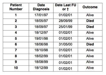
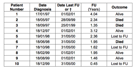
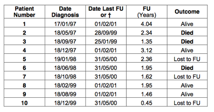
It is easiest to explain life table survival analysis with an example. Lets look at 10 patients who have been diagnosed with cancer. The date of diagnosis is shown in the 2nd column of the table below. Analysis was performed on 1/2/2001.
Patients who were alive at 1/2/2001, had this date inserted in the 3rd column (date last follow up). If the patient died, the date of death was inserted in the 3rd column. The 4th column indicates which patients died and which patients were alive:
 The data can also be shown in a graph:
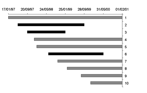
Patients who died are indicated in black and survivors in grey.
Next, the follow up between the two events (date of diagnosis and date of death / last follow up) is calculated for every patient:
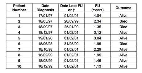
In total, there are 10 patients. All these patients have a follow up between 0 and 5 years. However, some patients have a follow up that is longer than others. This has to be taken into account if we want to calculate the probability of survival.
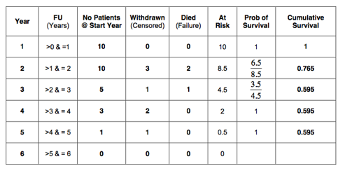
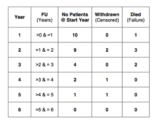
The probability of survival is calculated at yearly intervals (see table below). We started with 10 patients. Therefore, there were 10 patients at the beginning of year 1. From the table we can see that all patients had a follow up of more than 1 year. Therefore, at the start of the 2nd year there were still 10 patients.
Five patients had a follow up between 1 and 2 years. Two of these patients died and 3 patients were still alive at review. The 3 patients who were still alive have only been observed for part of the second year. They could still die during the remainder of that year. These 3 patients are called withdrawn from follow up.
Patients who have been withdrawn from follow up are also called ‘censored’; in other words the event of interest (death) was not observed. Similarly, patients are called ‘uncensored’ if the event of interest (death) was observed. So, in the 2nd year, 2 patients were uncensored and 3 patients were censored.
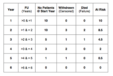
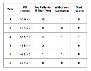
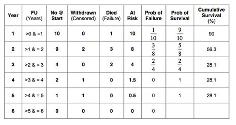
At the beginning of the 3rd year there were 5 patients left. 2 patients had a follow up between 2 and 3 years. One of these patients died (uncensored) and 1 patient withdrew from follow up (censored). Consequently, at the start of the 4th year there were only 3 patients left. 2 patients withdrew from follow up during the 4th year and none died. This left only 1 patient at the start of year 5. This patient had a follow up of just over 4 years and consequently withdrew during the 5th year. All these figures have been inserted in the table below:
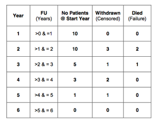 It must be clear that the number of patients at the start of a year, minus the patients withdrawn in that year minus the patients who died in that year make up the number of patients at the start of the next year. In other words: the number of patients at the start of a year minus the number censored minus the number uncensored in that year equals the number at the start of the next year. For example, at the first year: there were 10 patients at the start, minus 0 patients who withdrew, minus 0 patients who died in that year. This equals 10 patients at the start of year 2.
Or:
10 – 0 – 0 = 10
Similarly, for the 2nd year:
10 – 3 – 2 = 5
And the 3rd year:
5 – 1 – 1 = 3
For the 4th year:
3 – 2 – 0 = 1
And the 5th year:
1 – 1 = 0
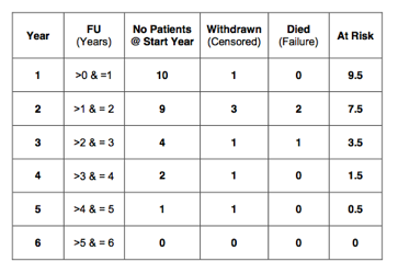
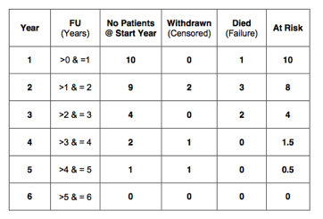
Patients who withdrew from follow up were observed for only part of that year. We know that they were alive at the date of last follow up and that the event of interest (death) has not occurred. However, there is a possibility that these patients might still die during the remainder of that year. We just don’t have enough follow up to be sure. So, these patients are only at risk of death for part of that year. In other words: the censored patients are at risk of the event of interest for only part of that year. On average, these patients will only have half the risk.
In the first year, no patients withdrew from follow up. Therefore, we will start with the 2nd year. In that year 3 patients withdrew from follow up. These 3 patients have only been at risk for half of the 2nd year. We can say that only 1.5 of these patients have been at risk of death. So, in total 8.5 patients (10 – 1.5) have been at risk of death during the 2nd year. This has been indicated in the 6th column in the table below. Similarly, 4.5 patients (5 – 0.5) were at risk in the 3rd year, 2 (3 – 1) in the 4th year, 0.5 (1 – 0.5) in the 5th year and 0 in the last year:
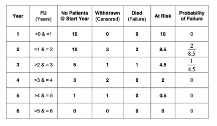
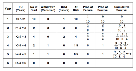
 The probability of the event of interest (death) equals:
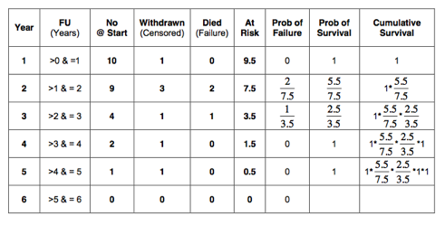
The probability of failure (death) has been calculated at yearly intervals and is indicated in the 7th column of the table below:
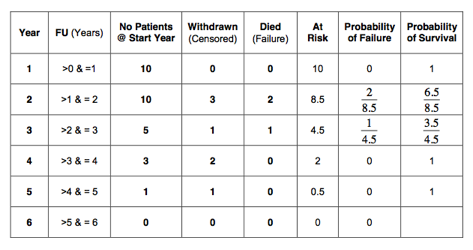
 The probability of survival is:
Probability (Survival) = 1 – Probability (Failure)
The probability of success (survival) has been calculated at yearly intervals and is shown in the 8th column in the table below:
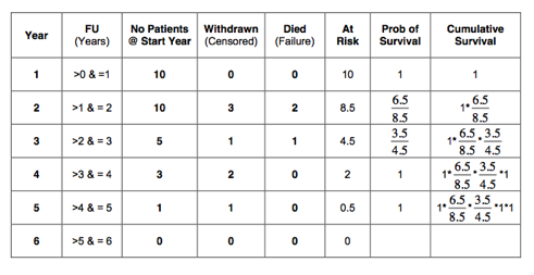
 The probability of surviving two years obviously depends on having survived the first year. Similarly, the probability on surviving 3 years depends on having survived year 1 and 2; and so on. As discussed, these dependent probabilities should be multiplied. Therefore, the cumulative survival should be calculated. Being a probability, the cumulative survival is a figure between 0 and 1 (or 0% and 100%). In this example the cumulative probability of
surviving the 1st year is 1;
the probability of surviving the 2nd year: ;
the third year: ;
the 4th year: ;
and in the 5th year:
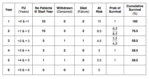
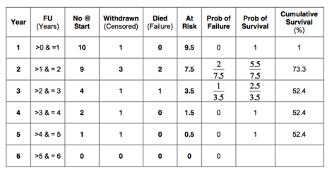
The cumulative survival in our example is shown in the last column of the table below:
 If we perform the calculation:
 Or in percentages:
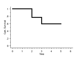
 The cumulative survival can also be plotted in a graph, as shown below.To indicate that the survival has been calculated at yearly intervals, the graph is stepped rather than smooth. The survival curve is stepped at yearly intervals in life table survival analysis:
 In the example, all patients who did not die were reviewed on 1st February 2001. In reality however, patients are lost to follow up. How to perform the analysis in this situation? Look at the example again, but now assume that patients number 5, 7 and 10 were lost to follow up. The last time they were seen was on 31st May 2000. At that time they were alive and well. What happened after is not known. This is summarised in the table below:
 As before, a table can be constructed that shows the number of patients at the start of each year, the number of patients who withdrew (censored) and the patients who died (uncensored):
 The censored patients are only at risk for part of the year. On average, they will have half the risk. The number of patients at risk per year has been calculated and is indicated in the 6th column of the table below:
 As before, calculate the probability of failure, probability of survival and the cumulative survival:
 Or in percentages:
 Therefore, the cumulative survival at 5 years is 52%, which is almost the same as calculated previously (60%). However, we have counted the patients lost to follow up as censored. In doing so, we have counted them as a success! It is however possible that these patients have died. We just don’t know (as they are lost to follow up). All we know is that they were alive on the 31st May 2000. They could have died the following day. What we have calculated is the cumulative survival at 5 years, whilst the 3 patients lost to follow up have been counted as a success. In other words, we have calculated the best-case scenario. So what is the worst-case scenario, when all patients lost to follow up are counted as failures (dead)? Summarised in a table:
 This time, count the patients lost to follow up as having died:
 As before, calculate the number of patients at risk:
 The probability of failure, probability of survival and cumulative survival have also been calculated and are summarised in the table below:
 Or in percentages:
 So, we have now calculated the best-case scenario and the worst-case scenario. The cumulative survival at 5 years is at best 52% and at worst 28%. The reality is probably somewhere in between these two values. The best- and worst-case scenarios survival curves are shown in one graph:
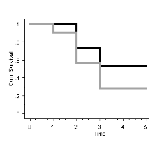 The best-case scenario is indicated in black and the worst-case scenario in grey. Patients who are censored are either lost to follow up, or the event of interest has not yet occurred. For patients who are lost to follow up, worse- and best-case scenarios can be calculated. In reality, the cumulative survival probably lies somewhere in between these two extremes.