Z-Scores
The mean height is different for children of different age. Children are growing and their height increases with age. It is important to know whether a child grows sufficiently as compared to its peers. Therefore, standardisation is required. Z-scores were introduced for this purpose. The child’s height is expressed as how many standard deviations it is above or below the mean.
Z-score =
The growth charts show that the average height for a twelve year old girl is 150 cm.
A child of average height has a z-score of 0:
Z-score =
What about twelve year old girl who is 160 cm?
Z-score =
The standard deviation can be estimated from the growth chart. It was shown that the mean + / – one standard deviation is between the 16th and 84th percentile. The 16th percentile for a twelve year old girl is approximately 142 cm (read from chart). Therefore, the standard deviation is 150 – 142 = 8 cm. Consequently, the Z-score of a 12 year old girls who is 160 cm is:
Z-score =
She is one and a quarter standard deviations above the mean for her age.
Similarly, a twelve year old girl who is 125 cm has a Z-score of:
Z-score =
She is more than 3 standard deviations below the average for her age.
Z-scores are very useful in follow up of children and comparing their growth rate with their peers. Assume a five year old child has a Z-score of -1 (one standard deviation below the average height for a five year old). If the child has a Z-score of -2 when 10 years old, the rate of growth has been less than its peers and this could indicate malnutrition or disease. But, if the child has a Z-score of 0 when 10 years old, the rate of growth has exceeded that of its peers. If the child has a Z-score of -1 when 10 years old, the rate of growth has been the same as its peers. The child however remains smaller than average and one standard deviation below the mean.
In summary, a change in Z-score indicates a difference in growth rate as compared to the normal population. An increase in Z-score indicates a growth rate greater than average and a decrease in Z-score a growth rate less than average. If the Z-score remains the same, the rate of growth is the same as the normal population.
T-Scores
Z-scores can also be used to express bone mineral density. The bone mineral density is referenced to the mean for that age:
A Z-score is the number of standard deviations the bone mineral density measurement is above or below the age-matched mean bone mineral density.
Z-score =
(BMD = bone mineral density)
However, to define osteoporosis the bone mineral density in a young normal is used as reference. This is the T-score:
A T-score is the number of standard deviations the bone mineral density measurement is above or below the young-normal mean bone mineral density.
T-score =
(BMD = bone mineral density)
The World Health Organisation defined osteoporosis / osteopenia in 1994. Four diagnostic categories were defined based on bone mineral density. The T-score, using young adult women as the referent group, defines the diagnostic categories:
- Normal: T-score -1 or above
- Osteopenia: T-score between -1 and -2.5
- Osteoporosis: T-score less than -2.5
- Severe osteoporosis: T-score less than -2.5 and fragility fracture
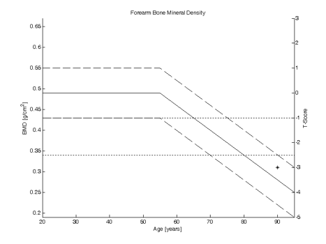
The graph below shows the forearm bone mineral density as function of the age:
 The left hand y-axis indicates the bone mineral density in gram per centimetre square. The corresponding T-score is based on the bone mineral density in a 20 year old and shown on the right hand y-axis. The solid line indicates the mean bone mineral density and the dashed lines one standard deviation away from the mean. Therefore, 68% of the people have a bone mineral density between the two dashed lines.
The two horizontal dotted lines show the osteopenia limit (T-score = -1) and the osteoporosis limit (t-score = -2.5). Z-scores are less commonly used than T-scores, but may be helpful in identifying persons who should undergo a work-up for secondary causes of osteoporosis. Z-scores and T-scores can be converted into each other using a reference table provided the age, gender, race and skeletal site are known.
Neither the Z-score not the T-score can predict fracture risk on its own. It is also necessary to know the age of the patient. Because T-scores and Z-scores can be converted into each other, fracture risk can be predicted with either.
Consider the patient in the graph below:
 Patient
Age: 70 years
Bone mineral density: 0.465 g/cm^2
Z-score: +1
Young normal (20 years)
Mean bone density: 0.49 g/cm^2
Standard deviation bone density: 0.49 – 0.43 = 0.06 g/cm^2
T-score:
WHO category: Normal
Also, the bone density measurement of the 90 years old lady with a fracture neck of femur:
 Patient
Age: 90 years
Bone mineral density: 0.31 g/cm^2
Z-score: ≈ + 0.5
Young normal (20 years)
Mean bone density: 0.49 g/cm^2
Standard deviation bone density: 0.49 – 0.43 = 0.06 g/cm^2
T-score:
WHO category: Severe osteoporosis
In JGR / R:
The Normal distribution is central to parametric statistics. Normally distributed data are commonly described in terms of their mean and standard deviation. It has been demonstrated that people’s heights can be regarded as a Normal distribution. It is important to distinguish between the sample descriptives (mean and standard deviation) and population descriptives (mean μ and standard deviation σ).
The data set heights.rda contains the heights of two groups of people. To obtain the descriptives is easy in JGR:
Or directly in the console:
descriptive.table(vars = d(Group1,Group2),data= heights, func.names =c(“Mean”,”St. Deviation”,”Valid N”,”Minimum”,”Maximum”))
$`strata: all cases `
Mean St. Deviation Valid N Minimum Maximum
Group1 164.9281 4.888238 1000 147.5271 179.0782
Group2 178.5239 15.284486 1000 125.4151 232.9516
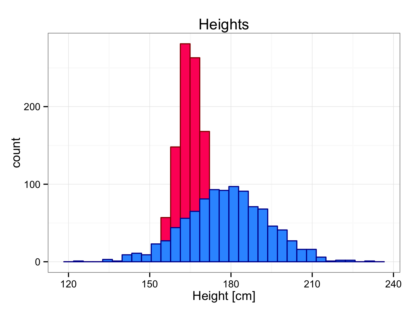
To obtain a histogram showing both group of data, Group1 in red and Group2 in blue is straight forward in plot builder, or alternatively directly in the console:
ggplot() + theme_bw() + geom_histogram(aes(y = ..count..,x = Group1),data=heights,colour = “#990000″,fill = “#ff0066″) + geom_histogram(aes(x = Group2),data=heights,colour = “#000099″,fill = “#3399ff”) +xlab(label = “Height [cm]”) + ggtitle(label = “Heights”)
 The Z-score can be calculated by the following equation:
So, the Z-score of a person in Group 2 whose height is 200 cm is:
The positive Z score indicates the height is above the mean; by 1.41 standard deviations. R can be used to calculate the probability of having a height of 200 cm or less using the pnorm function:
pnorm(1.41)
[1] 0.9207302
So, 92%.
If the probability of having a height of more than or equal to 210 cm is required:
1-pnorm(2.06)
[1] 0.01969927
Or 2%.
The probability of the height being between 200 and 210 cm is:
pnorm(2.06)-pnorm(1.41)
[1] 0.05957057
Or 6%.