circlize 1 can be used to make chromosome ideograms. The example below uses the hg19 assembly (GRCh37) as reference. However, the newer (hg38 / GRCh38) can also be downloaded, manipulated and used instead (see below). It is important to use the appropriate reference assembly when working with genomic data.
For the examples below to work, the dplyr 2 and stringr 3 packages should also be installed and loaded for a default plot with the hg19 assembly:
library(circlize)
library(dplyr)
library(stringr)
# https://jokergoo.github.io/circlize_book/book/initialize-genomic-plot.html
# https://cran.r-project.org/web/packages/circlize/circlize.pdf
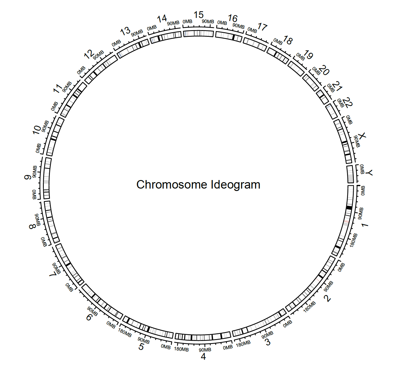
# create an ideogram
circos.initializeWithIdeogram()
# the plot names the chromosome numeric, but the internal names have ‘chr’ in front of them
# for index use chr1 etc
# add text:
text(0, 0, “Chromosome Ideogram”, cex = 1)
# info:
circos.info()
All your sectors:
[1] “chr1″ “chr2″ “chr3″ “chr4″ “chr5″ “chr6″ “chr7″ “chr8″ “chr9″ “chr10″ “chr11″
[12] “chr12″ “chr13″ “chr14″ “chr15″ “chr16″ “chr17″ “chr18″ “chr19″ “chr20″ “chr21″ “chr22″
[23] “chrX” “chrY”
All your tracks:
[1] 1 2
Your current sector.index is chrY
Your current track.index is 2
# clear the plotting
circos.clear()
The default ideogram is hg19, but this can be changed with the species argument. However, circos.initializeWithIdeogram(species = “hg38″) doesn’t work as there are too many unmapped regions. The hg38 cytoband can be downloaded from:
http://hgdownload.cse.ucsc.edu/goldenpath/hg38/database/
Put it on the desktop and read it in:
cytoband.df.1 <- read.table(“~/Desktop/cytoBand_hg38.txt”, colClasses = c(“character”, “numeric”, “numeric”, “character”, “character”), sep = “\t”)
# Remove the unmapped areas: remove chromosome names that end in _alt or _random or start with chrUn:
cytoband.df.2 <- cytoband.df.1 %>%
dplyr::filter(!str_detect(V1, “chrUn”)) %>%
dplyr::filter(!str_detect(V1, “_alt”)) %>%
dplyr::filter(!str_detect(V1, “_random”))
circos.initializeWithIdeogram(cytoband.df.2)
circos.clear()

By default, all chromosomes are displayed, but this can be changed with the index:
circos.initializeWithIdeogram(cytoband.df.2, chromosome.index = paste0(“chr”, c(3,5,2,8)))
text(0, 0, “subset of chromosomes”, cex = 1)
circos.clear()

Where to start can be set with circos.par:
circos.par(“start.degree” = 90)
circos.initializeWithIdeogram(cytoband.df.2)
circos.clear()
text(0, 0, “‘start.degree’ = 90″, cex = 1)

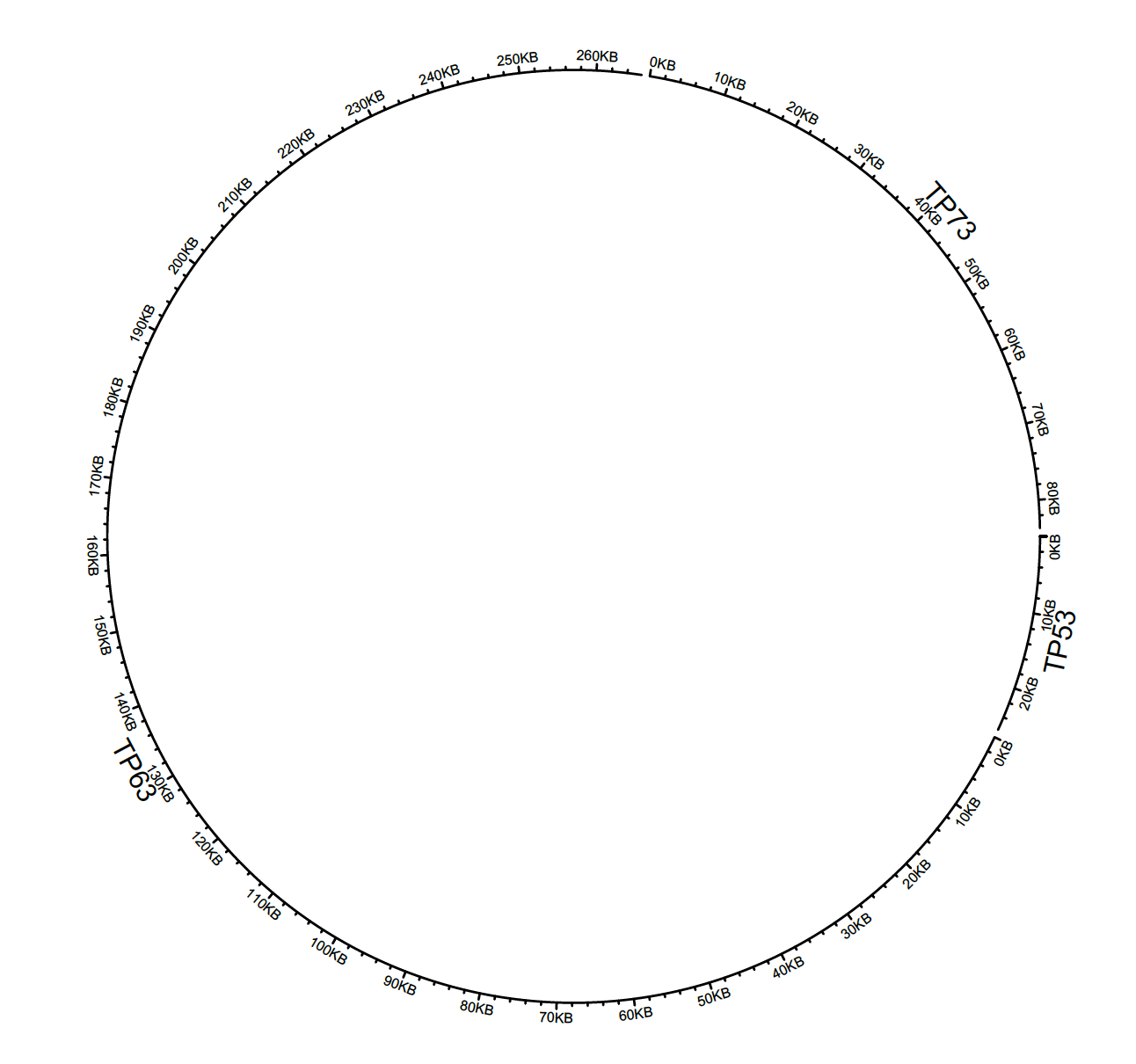
To plot different genes:
df = data.frame(
name = c(“TP53″, “TP63″, “TP73″),
start = c(7565097, 189349205, 3569084),
end = c(7590856, 189615068, 3652765))
circos.genomicInitialize(df)
circos.clear()
Custom plot:
tp_family = readRDS(system.file(package = “circlize”, “extdata”, “tp_family_df.rds”))
head(tp_family)
gene start end transcript exon
1 TP53 7565097 7565332 ENST00000413465.2 7
2 TP53 7577499 7577608 ENST00000413465.2 6
3 TP53 7578177 7578289 ENST00000413465.2 5
4 TP53 7578371 7578554 ENST00000413465.2 4
5 TP53 7579312 7579590 ENST00000413465.2 3
6 TP53 7579700 7579721 ENST00000413465.2 2
# build track
circos.genomicInitialize(tp_family)
# give colours to different genes:
circos.track(ylim = c(0, 1),
bg.col = c(“#FF000040″, “#00FF0040″, “#0000FF40″),
bg.border = NA, track.height = 0.05)
# add transcripts
n = max(tapply(tp_family$transcript, tp_family$gene, function(x) length(unique(x))))
circos.genomicTrack(tp_family, ylim = c(0.5, n + 0.5),
panel.fun = function(region, value, …) {
all_tx = unique(value$transcript)
for(i in seq_along(all_tx)) {
l = value$transcript == all_tx[i]
# for each transcript
current_tx_start = min(region[l, 1])
current_tx_end = max(region[l, 2])
circos.lines(c(current_tx_start, current_tx_end),
c(n – i + 1, n – i + 1), col = “#CCCCCC”)
circos.genomicRect(region[l, , drop = FALSE], ytop = n – i + 1 + 0.4,
ybottom = n – i + 1 – 0.4, col = “orange”, border = NA)
}
}, bg.border = NA, track.height = 0.4)
circos.clear()

Custom zoomed plot:
# zooming into chromosomes
extend_chromosomes = function(bed, chromosome, prefix = “zoom_”) {
zoom_bed = bed[bed[[1]] %in% chromosome, , drop = FALSE]
zoom_bed[[1]] = paste0(prefix, zoom_bed[[1]])
rbind(bed, zoom_bed)
}
# use the downloaded hg38 assembly from above:
head(cytoband.df.2)
V1 V2 V3 V4 V5
1 chr1 0 2300000 p36.33 gneg
2 chr1 2300000 5300000 p36.32 gpos25
3 chr1 5300000 7100000 p36.31 gneg
4 chr1 7100000 9100000 p36.23 gpos25
5 chr1 9100000 12500000 p36.22 gneg
6 chr1 12500000 15900000 p36.21 gpos50
# chromosome names
chromosome <- unique(cytoband.df.2$V1)
chromosome
[1] “chr1″ “chr10″ “chr11″ “chr12″ “chr13″ “chr14″ “chr15″ “chr16″ “chr17″ “chr18″ “chr19″
[12] “chr2″ “chr20″ “chr21″ “chr22″ “chr3″ “chr4″ “chr5″ “chr6″ “chr7″ “chr8″ “chr9″
[23] “chrM” “chrX” “chrY”
# chromosome length
chromosome.length <- cytoband.df.2 %>% dplyr::group_by(V1) %>% summarise(max = max(V3))
chromosome.length
# A tibble: 25 x 2
V1 max
<chr> <dbl>
1 chr1 248956422
2 chr10 133797422
3 chr11 135086622
4 chr12 133275309
5 chr13 114364328
6 chr14 107043718
7 chr15 101991189
8 chr16 90338345
9 chr17 83257441
10 chr18 80373285
# … with 15 more rows
# length of 1st and second chromosome
chromosome.1.length <- as.numeric(chromosome.length[1,2])
chromosome.2.length <- as.numeric(chromosome.length[12,2])
# add all chromosome lengths to a vector and add again chr1 and chr2; used for zooming
x_range <- c(chromosome.length$max, chromosome.1.length, chromosome.2.length)
names(x_range) <- c(chromosome.length$V1, “chr1″, “chr2″)
# calculate sector width
normal_chr_index = 1:25
zoomed_chr_index = 26:27
# normalize in normal chromsomes and zoomed chromosomes separately
sector.width = c(x_range[normal_chr_index] / sum(x_range[normal_chr_index]),
x_range[zoomed_chr_index] / sum(x_range[zoomed_chr_index]))
### create the plot
circos.par(start.degree = 90)
circos.initializeWithIdeogram(extend_chromosomes(cytoband.df.2, c(“chr1″, “chr2″)), sector.width = sector.width)
# add a new track:
bed = generateRandomBed(500)
circos.genomicTrack(extend_chromosomes(bed, c(“chr1″, “chr2″)),
panel.fun = function(region, value, …) {
circos.genomicPoints(region, value, pch = 16, cex = 0.3)
})
Note: 1 point is out of plotting region in sector ‘chr9′, track ‘3’.
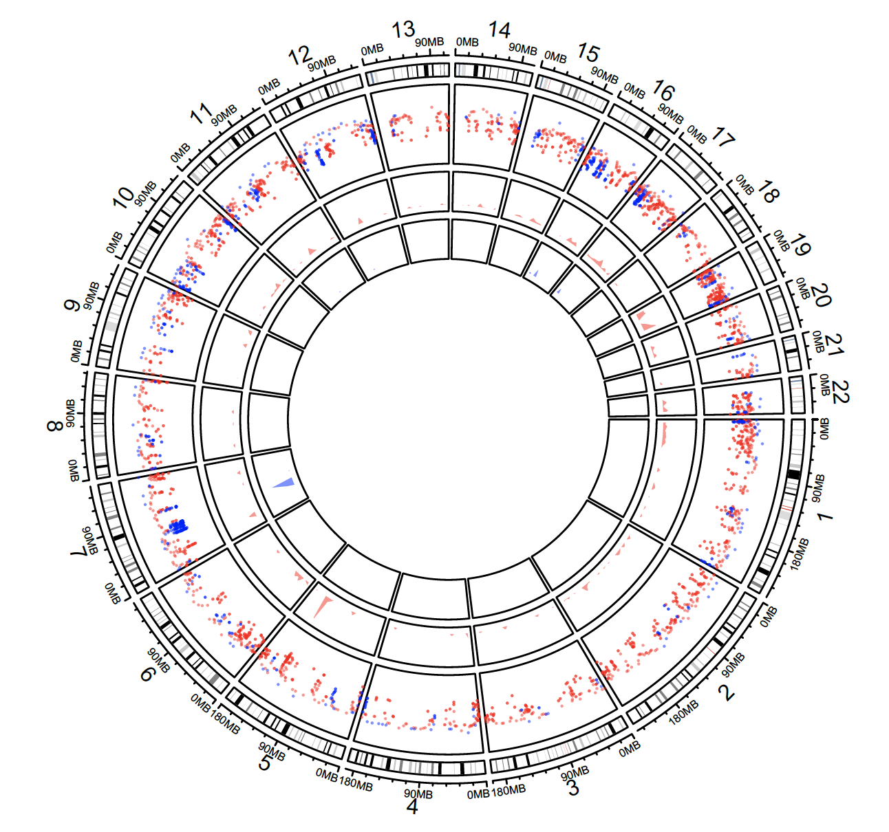
#Add a link from original chromosome to the zoomed chromosome (Figure 8.7).
circos.link(“chr1″, get.cell.meta.data(“cell.xlim”, sector.index = “chr1″),
“zoom_chr1″, get.cell.meta.data(“cell.xlim”, sector.index = “zoom_chr1″),
col = “#00000020″, border = NA)
circos.clear()

High level genomic functions
# hg19 (default)
circos.initializeWithIdeogram(plotType = c(“labels”, “axis”))
circos.track(ylim = c(0, 1)) # this puts a blank track in
circos.genomicIdeogram() # put ideogram as the third track
circos.genomicIdeogram(track.height = 0.1)
circos.clear()

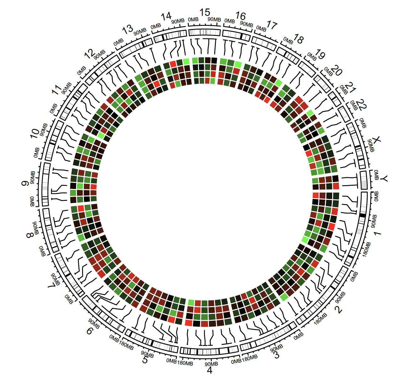
Heatmap
circos.initializeWithIdeogram()
bed = generateRandomBed(nr = 100, nc = 4)
col_fun = colorRamp2(c(-1, 0, 1), c(“green”, “black”, “red”))
circos.genomicHeatmap(bed, col = col_fun, side = “inside”, border = “white”)
circos.clear()
Labels
circos.initializeWithIdeogram()
bed = generateRandomBed(nr = 50, fun = function(k) sample(letters, k, replace = TRUE))
bed[1, 4] = “aaaaa”
circos.genomicLabels(bed, labels.column = 4, side = “inside”)

Density and rainfall plots
load(system.file(package = “circlize”, “extdata”, “DMR.RData”))
circos.initializeWithIdeogram(chromosome.index = paste0(“chr”, 1:22))
bed_list = list(DMR_hyper, DMR_hypo)
circos.genomicRainfall(bed_list, pch = 16, cex = 0.4, col = c(“#FF000080″, “#0000FF80″))
circos.genomicDensity(DMR_hyper, col = c(“#FF000080″), track.height = 0.1)
circos.genomicDensity(DMR_hypo, col = c(“#0000FF80″), track.height = 0.1)