Equation of Time | Stats Book

Introduction

Noon is 12 o’clock at daytime. However, the chronological time does not coincide with solar noon, when the sun reaches its highest point in the sky. This is due to three factors:

Longitude
The equation of time
Daylight savings

In this section, daylight savings are not taken into consideration. But the other factors are explored to calculate the time of local solar noon. Furthermore, the timing of sun rise and sun set are estimated and graphically presented.

Longitude correction

Latitude and longitude are used to describe a location on earth. They can be expressed in degrees, minutes and seconds (DMS notation) or in digital degrees (DD notation). In software programs, it is easiest to use the DD notation. It is however straight forward to convert from one format to the other using the following functions:

R download: convert_dms_dd

R download: convert_dd_dms

In Britain, the time corresponds to the time at Greenwich (GMT) at the null meridian. When located to the east, solar time is earlier than GMT and to the west later. To calculate solar time, it is necessary to correct for this difference in longitude. The correction required is 240 seconds for every degree (1 day per 360 degrees = 24 × 60 × 60 / 360 = 240 seconds per degree).

Equation of Time

The equation of time describes the difference between mean solar time (chronological time as shown on the clock) and the apparent solar time (as shown on a sundial). This is mainly caused by two factors:

The obliquity of the ecliptic plane, which is inclined by approximately 23 degrees relative to the earth’s equator
The eccentricity of the earth’s orbit around the sun

The effect of both factors can be summarised in the following formula (or equation of time) with reasonable accuracy (other approximations have been described):

$Correction = 9.87 \times sin(2 \times B) - 7.53 \times cos(B)-1.5 \times sin(B)$

where,

$B = 2 \times \pi \times (Day Number - 81) / 365$

Day number 81 is 22nd March.

For leap years, divide be 366

R download: equation_of_time

With this formula, the timing of solar noon can be estimated. Subsequently, if the declination of the sun is know, the timing of sun set and sun rise can also be estimated as described below.

Sun declination

The declination of the sun is estimated using the following formula:

$Declination = 23.45 \times sin( \frac{2 \times \pi}{{365}} \times (DayNumber + 284))$

Day 284 is 11th October

R download: sun_declination

Sun rise formula

Knowing the solar declination on a particular day, the sun rise and sun set times can be estimated using the following formula (all angles in radians):

$w = \frac{sin(Altitude[rad]) - sin(Latitude[rad]) \times sin(Declination[rad])}{cos(Latitude[rad])) \times cos(Declination[rad]))}$

where the declination can be estimated using the formula described above. To convert to radians:

$Declination[rad] = Declination[degrees] \times \frac{\pi}{180}$

To convert the latitude to radians:

$Latitude[rad] = Latitude[degrees] \times \frac{\pi}{180}$

If the altitude is zero, the formula gives the timing that the centre of the solar disc is at the horizon. To estimate when the top of the solar disc reaches the horizon, subtract 16 arc minutes for the semi-diameter of the solar disc and 34 arc minutes for atmospheric refraction (different under different atmospheric conditions). In total, subtract 50 arc minutes:

$Altitude[rad] = -\frac{50}{60} \times \frac{\pi}{180} + s \times \frac{\pi}{180}$

The parameter s corrects for the solar altitude at different timings. For sun rise and sun set, s should be set at zero. Twilights can be estimated by varying s:

s = 0 sun rise / sun set
s = -6 civil twilight
s = -12 nautical twilight
s = -18 astronomical twilight

The formula returns a value w, that can be converted to an hour angle (in radians) by taking the arccos (inverse function of the cosine) of w:

$HourAngle[rad] = arccos(w)$

which in turn can be converted to degrees:

$HourAngle[degrees] = HourAngle[rad] \times \frac{180}{\pi}$

To calculate the sun rise and sun set times before and after solar noon (in seconds):

$RiseSet[seconds] = HourAngle[degrees] \times 240$

(1 day per 360 degrees = 24 × 60 × 60 / 360 = 240 seconds per degree).

Sun rise can be found by:

$SunRise = SolarNoon - RiseSet[seconds]$

and sun set:

$SunSet = SolarNoon + RiseSet[seconds]$

R download: sun_rise_formula

Graphical presentation

To allow visualisation in R, the following packages should be installed as described:

dplyR package: 1, to manipulate data frames
ggplot2 package: 2, to create plots
lubridate package: 3, to work with dates

The following functions, as described above, should be copied and pasted into R and executed as described:

Location

As example the location is set at the Robert Jones and Agnes Hunt Orthopaedic Hospital NHS Foundation Trust. The coordinates are (DMS):

Longitude: 3 degrees, 1 minute and 57.8 seconds West

Latitude: 52 degrees, 53 minutes and 3.7 seconds North

To convert to DD and show the result (North and East are +, South and West are -):

library(dplyr)
library(ggplot2)
library(lubridate)

convert_dms_dd <- function(deg, min, sec){
result <- deg + min / 60 + sec / 3600
}

longitude <- convert_dms_dd(3, 1, 57.8)
# East is negative, so make negative:
longitude <- – longitude

latitude <- convert_dms_dd(52, 53, 3.7)

# show the values:
longitude
[1] -3.032722
latitude
[1] 52.88436

Create a vector of day numbers:

days <- rep(1:365, by = 1)

Load the formulas defined above:

sun_rise_formula <- function(day_number, declination, latitude, s){
# altitude correction needed; otherwise centre of the sun disk.
# – 16 arc minutes for semi-diameter of the sun disk
# horizontal refraction: – 34 arc minutes
# total – 50 arc minutes = – 50 / 60 deg
altitude_rad <- – 50 / 60 * pi / 180 + s * pi / 180
latitude_rad <- latitude * pi / 180
declination_rad <- declination * pi / 180
w <- (sin(altitude_rad) – (sin(latitude_rad) * sin(declination_rad))) /
(cos(latitude_rad) * cos(declination_rad))
hour_angle_rad <- acos(w)
hour_angle <- hour_angle_rad * 180 / pi
rise_set_seconds <- hour_angle * 240
result <- rise_set_seconds
}
sun_declination <- function(day_number){
result <- 23.45 * sin(2 * pi / 365 * (day_number + 284))
}
equation_of_time <- function(day_number){
# day_number is the number of the day in the year
# 81 is the 22nd March
# B in radians
B <- 2 * pi * (day_number – 81) / 365
# correction in minutes
result <- 9.87 * sin(2 * B) – 7.53 * cos(B) – 1.5 * sin(B)
# correction in seconds
result <- result * 60
}

Calculate the correction (equation of time), the solar declination and the time of sun rise / sun set before / after solar noon:

correction <- equation_of_time(day_number = days)
declination <- sun_declination(day_number = days)
rise_set_seconds <- sun_rise_formula(day_number = days, declination = declination, latitude = latitude, s = 0)

Convert to a data frame (called solar_time):

solar_time <- data.frame(“day” = days, “correction” = correction, “declination” = declination, “rise_set” = rise_set_seconds)

Calculate the solar altitude from the solar declination and add to the data frame:

solar_time$altitude <- 90 – latitude + solar_time$declination

Add the longitude correction and the total time correction (longitude and equation of time) to the data frame:

solar_time$longitude_correction <- longitude * 240
solar_time$total_correction <- solar_time$longitude_correction + solar_time$correction

Also add the start time of the day and the time of chronological noon to the data frame:

solar_time$start <- ymd_hms(“2017-12-31 00:00:00″, tz = “GMT”) + ddays(solar_time$day)
solar_time$noon <- ymd_hms(“2017-12-31 12:00:00″, tz = “GMT”) + ddays(solar_time$day)

Calculate apparent solar noon (as seen on a sun dial) and add to the data frame:

solar_time$noon_apparent <- solar_time$noon – dseconds(solar_time$total_correction)

Calculate sun set, sun rise and the total day length and add to the data frame:

solar_time$sun_rise <- solar_time$noon_apparent – dseconds(solar_time$rise_set)
solar_time$sun_set <- solar_time$noon_apparent + dseconds(solar_time$rise_set)
solar_time$day_length <- solar_time$sun_set – solar_time$sun_rise

Similarly, calculate the timings of civil, nautical and astronomical twilight and add to the data frame:

# add civil twilight s = – 6
# add nautical twilight s = – 12
# add astronomical twilight, s = – 18
solar_time$civil_seconds <- sun_rise_formula(day_number = days, declination = declination, latitude = latitude, s = – 6)
solar_time$nautical_seconds <- sun_rise_formula(day_number = days, declination = declination, latitude = latitude, s = – 12)
solar_time$astro_seconds <- sun_rise_formula(day_number = days, declination = declination, latitude = latitude, s = – 18)
Warning message:
In acos(w) : NaNs produced
solar_time$civil_rise <- solar_time$noon_apparent – dseconds(solar_time$civil_seconds)
solar_time$civil_set <- solar_time$noon_apparent + dseconds(solar_time$civil_seconds)
solar_time$nautical_rise <- solar_time$noon_apparent – dseconds(solar_time$nautical_seconds)
solar_time$nautical_set <- solar_time$noon_apparent + dseconds(solar_time$nautical_seconds)
solar_time$astro_rise <- solar_time$noon_apparent – dseconds(solar_time$astro_seconds)
solar_time$astro_set <- solar_time$noon_apparent + dseconds(solar_time$astro_seconds)

The warning message shows that NaNs are introduced when there is no astronomical twilight in the height of summer.

The data frame is now complete and can be reviewed with:

str(solar_time)
head(solar_time)
tail(solar_time)
solar_time

Output omitted for brevity.

Retrieve the following from the data frame and define them for later use:

earliest sun rise
latest sun rise
earliest sun set
latest sun set
shortest day
longest day

earliest_sun_rise <- solar_time %>%
dplyr::mutate(sun_rise_hour = hour(sun_rise) + minute(sun_rise) / 60 + second(sun_rise) / 3600) %>%
dplyr::filter(sun_rise_hour == min(sun_rise_hour))

latest_sun_rise <- solar_time %>%
dplyr::mutate(sun_rise_hour = hour(sun_rise) + minute(sun_rise) / 60 + second(sun_rise) / 3600) %>%
dplyr::filter(sun_rise_hour == max(sun_rise_hour))

earliest_sun_set <- solar_time %>%
dplyr::mutate(sun_set_hour = hour(sun_set) + minute(sun_set) / 60 + second(sun_set) / 3600) %>%
dplyr::filter(sun_set_hour == min(sun_set_hour))

latest_sun_set <- solar_time %>%
dplyr::mutate(sun_set_hour = hour(sun_set) + minute(sun_set) / 60 + second(sun_set) / 3600) %>%
dplyr::filter(sun_set_hour == max(sun_set_hour))

shortest_day <- solar_time %>%
dplyr::filter(day_length == min(day_length))

longest_day <- solar_time %>%
dplyr::filter(day_length == max(day_length))

earliest_sun_rise
day 168, 17/06
latest_sun_rise
day 364, 30/12
earliest_sun_set
day 346, 12/12
latest_sun_set
day 176, 25/6
shortest_day
day 355, 21/12
longest_day
day 172, 21/06

Output omitted, but summarised for readability.

Although the longest day is 21st June, the earliest sun rise is a few days earlier (17th June) and the latest sun set a few days later ((25th June). Similarly, around the shortest day (21st December) the latest sun rise is a few days later (30th of December) and the earliest sun set a few days earlier (12th December). This is better shown graphically in a plot that follows later.

Equation of time

It is now straight forward to plot the equation of time with ggplot2 2:

dev.new()
solar_time %>%
ggplot(aes(x = day, y = correction)) +
geom_line(colour = “blue”) +
scale_x_continuous(“Day Number”) +
scale_y_continuous(“Correction [seconds]”) +
ggtitle(“Equation of Time”) +
theme_bw()

Or add the current day to the plot:

dev.new()
solar_time %>%
ggplot(aes(x = day, y = correction)) +
geom_line(colour = “blue”) +
geom_point(data = subset(solar_time, solar_time$day == yday(now(tzone = “GMT”))), aes(x = day, y = correction), colour = “black”) +
geom_text(data = subset(solar_time, solar_time$day == yday(now(tzone = “GMT”))), aes(x = day, y = correction), label = today(), hjust = 1.1) +
scale_x_continuous(“Day Number”) +
scale_y_continuous(“Correction [seconds]”) +
ggtitle(“Equation of Time”) +
theme_bw()

To show a plot of the sun rise in red, sun set in orange and day length in green:

dev.new()
solar_time %>%
ggplot() +
geom_line(aes(x = day, y = (sun_rise – start)), colour = “red”) +
geom_line(aes(x = day, y = (sun_set – start)), colour = “orange”) +
geom_line(aes(x = day, y = day_length), colour = ‘darkgreen’) +
geom_vline(xintercept = longest_day$day, colour = “darkgreen”) +
geom_vline(xintercept = shortest_day$day, colour = “darkgreen”) +
geom_vline(xintercept = earliest_sun_rise$day, colour = “red”, linetype = 2) +
geom_vline(xintercept = latest_sun_rise$day, colour = “red”, linetype = 2) +
geom_vline(xintercept = earliest_sun_set$day, colour = “orange”, linetype = 2) +
geom_vline(xintercept = latest_sun_set$day, colour = “orange”, linetype = 2) +
ggtitle(“Sun Rise (red), Sun Set (orange) and Day Length (green)”) +
scale_x_continuous(“Day Number”, breaks = c(1, 100, latest_sun_set$day, longest_day$day, earliest_sun_rise$day, 200, 300, latest_sun_rise$day, shortest_day$day, earliest_sun_set$day), limits = c(0, 385)) +
geom_text(data = latest_sun_set, aes(x = day, y = 10, label = date(start)), colour = “orange”, hjust = – 0.1) +
geom_text(data = earliest_sun_rise, aes(x = day, y = 10, label = date(start)), colour = “red”, hjust = 1.1) +
geom_text(data = earliest_sun_set, aes(x = day, y = 10, label = date(start)), colour = “orange”, hjust = 1.1) +
geom_text(data = latest_sun_rise, aes(x = day, y = 10, label = date(start)), colour = “red”, hjust = – 0.1) +
geom_text(data = longest_day, aes(x = day, y = 17.5 , label = date(start)), colour = “darkgreen”, hjust = – 0.1) +
geom_text(data = shortest_day, aes(x = day, y = 17.5, label = date(start)), colour = “darkgreen”, hjust = – 0.1) +
scale_y_continuous(“Hours after Midnight”) +
theme_bw() +
theme(axis.text.x=element_text(angle = 90, hjust = 0, vjust = 0)) # after theme_bw call otherwise it doesnt’ work!

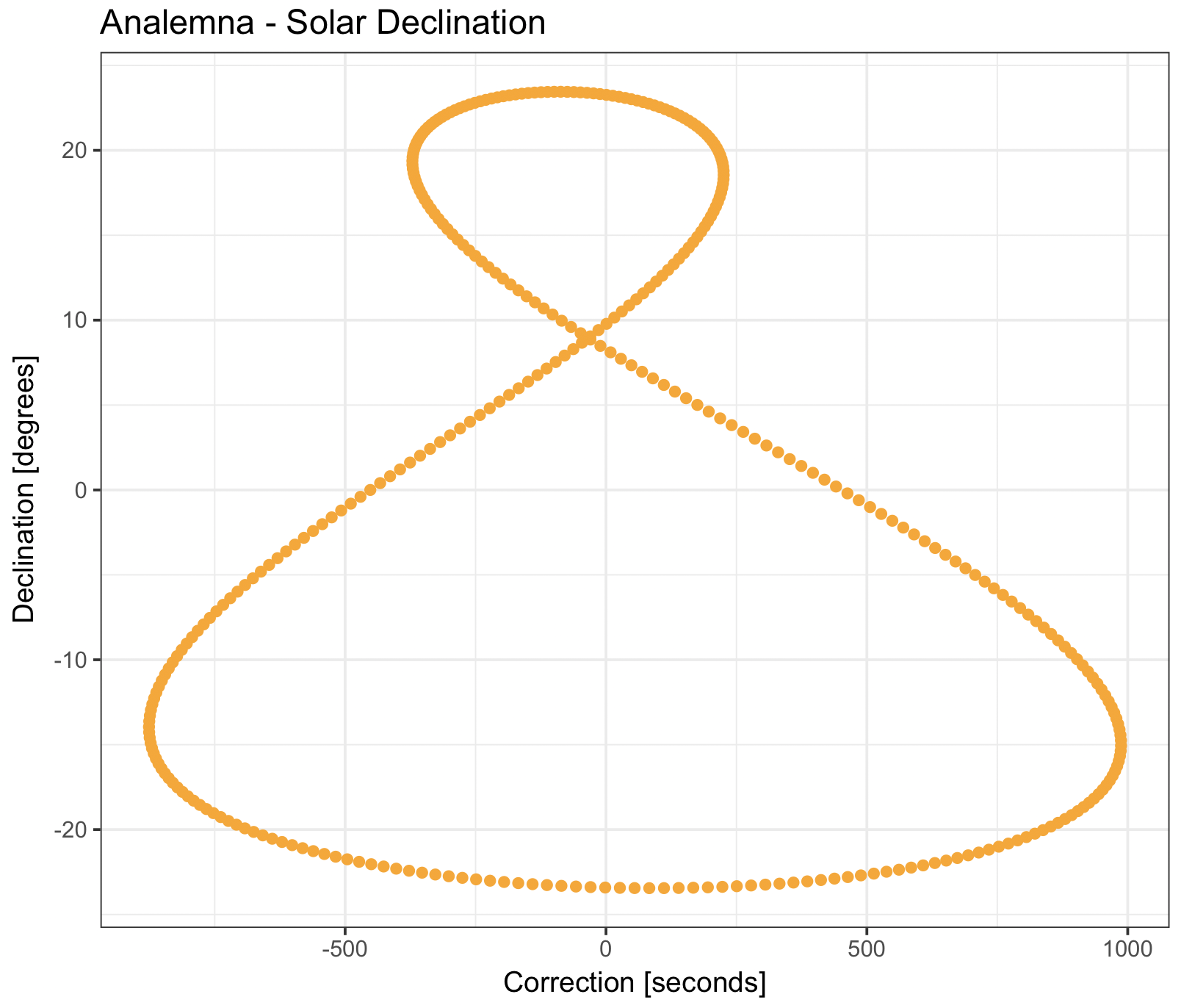
An analemna, shows the position of the sun in the sky every day at midday (chronological noon):

dev.new()
solar_time %>%
ggplot(aes(x = correction, y = declination)) +
geom_point(colour = “orange”) +
scale_x_continuous(“Correction [seconds]”) +
scale_y_continuous(“Declination [degrees]”) +
ggtitle(“Analemna – Solar Declination”) +
theme_bw()

Annotate different days on the plot:

dev.new()
solar_time %>%
ggplot(aes(x = correction, y = declination)) +
geom_point(colour = “grey”) +
scale_x_continuous(“Correction [seconds]”) +
scale_y_continuous(“Declination [degrees]”, limits = c(-25, 25)) +
ggtitle(“Analemna – Solar Declination”) +
# geom_text(data = subset(solar_time, solar_time$day == 1), aes(x = correction, y = declination, label = day), vjust = 2) +
# geom_point(data = subset(solar_time, solar_time$day == 1), aes(x = correction, y = declination), colour = “black”) +
geom_text(data = longest_day, aes(x = correction, y = declination, label = day), colour = “darkgreen”, vjust = – 1) +
geom_point(data = longest_day, aes(x = correction, y = declination), colour = “darkgreen”) +
geom_text(data = shortest_day, aes(x = correction, y = declination, label = day), colour = “darkgreen”, vjust = 2) +
geom_point(data = shortest_day, aes(x = correction, y = declination), colour = “darkgreen”) +
geom_text(data = latest_sun_set, aes(x = correction, y = declination, label = day), colour = “orange”, hjust = 0.7, vjust = 2) +
geom_point(data = latest_sun_set, aes(x = correction, y = declination), colour = “orange”) +
geom_text(data = latest_sun_rise, aes(x = correction, y = declination, label = day), colour = “red”, hjust = 0.5, vjust = 2) +
geom_point(data = latest_sun_rise, aes(x = correction, y = declination), colour = “red”) +
geom_text(data = earliest_sun_set, aes(x = correction, y = declination, label = day), colour = “orange”, vjust = 2) +
geom_point(data = earliest_sun_set, aes(x = correction, y = declination), colour = “orange”) +
geom_text(data = earliest_sun_rise, aes(x = correction, y = declination, label = day), colour = “red”, hjust = 0.1 , vjust = 2) +
geom_point(data = earliest_sun_rise, aes(x = correction, y = declination), colour = “red”) +
geom_point(data = subset(solar_time, solar_time$day == 104), aes(x = correction, y = declination), colour = “black”) +
geom_text(data = subset(solar_time, solar_time$day == 104), aes(x = correction, y = declination, label = day), hjust = 0, vjust = 2) +
geom_point(data = subset(solar_time, solar_time$day == 241), aes(x = correction, y = declination), colour = “black”) +
geom_text(data = subset(solar_time, solar_time$day == 241), aes(x = correction, y = declination, label = day), hjust = 0.2, vjust = -1) +
# add equinox in blue, table shows equinox on 20th March: day 79 and 23rd September day 266
geom_text(data = subset(solar_time, solar_time$day == 79), aes(x = correction, y = declination, label = day), colour = “blue”, hjust = – 0.3, vjust = 1) +
geom_point(data = subset(solar_time, solar_time$day == 79), aes(x = correction, y = declination), colour = “blue”) +
geom_text(data = subset(solar_time, solar_time$day == 266), aes(x = correction, y = declination, label = day), colour = “blue”, hjust = – 0.2, vjust = 0) +
geom_point(data = subset(solar_time, solar_time$day == 266), aes(x = correction, y = declination), colour = “blue”) +
# add the extreme corrections:
geom_point(data = subset(solar_time, solar_time$day == 44), aes(x = correction, y = declination), colour = “salmon”) +
geom_text(data = subset(solar_time, solar_time$day == 44), aes(x = correction, y = declination, label = day), colour = “salmon”, hjust = – 0.5, vjust = 0) +
geom_point(data = subset(solar_time, solar_time$day == 303), aes(x = correction, y = declination), colour = “salmon”) +
geom_text(data = subset(solar_time, solar_time$day == 303), aes(x = correction, y = declination, label = day), colour = “salmon”, hjust = 1.4, vjust = 0) +
theme_bw()

The plot is easier to read with text:

dev.new()
solar_time %>%
ggplot(aes(x = correction, y = declination)) +
geom_point(colour = “grey”) +
scale_x_continuous(“Correction [seconds]”) +
scale_y_continuous(“Declination [degrees]”, limits = c(- 30, 30)) +
ggtitle(“Analemna – Solar Declination”) +
# geom_text(data = subset(solar_time, solar_time$day == 1), aes(x = correction, y = declination, label = day), vjust = 2) +
# geom_point(data = subset(solar_time, solar_time$day == 1), aes(x = correction, y = declination), colour = “black”) +
geom_text(data = longest_day, aes(x = correction, y = declination), colour = “darkgreen”, label = “longest\nday”, vjust = – 0.5) +
geom_point(data = longest_day, aes(x = correction, y = declination), colour = “darkgreen”) +
geom_text(data = shortest_day, aes(x = correction, y = declination), colour = “darkgreen”, label = “shortest\nday”, vjust = 1.5) +
geom_point(data = shortest_day, aes(x = correction, y = declination), colour = “darkgreen”) +
geom_text(data = latest_sun_set, aes(x = correction, y = declination), colour = “orange”, label = “latest\nsun set”, hjust = 0.7, vjust = 1.5) +
geom_point(data = latest_sun_set, aes(x = correction, y = declination), colour = “orange”) +
geom_text(data = latest_sun_rise, aes(x = correction, y = declination), colour = “red”, label = “latest\nsun rise”, hjust = 0.5, vjust = 1.5) +
geom_point(data = latest_sun_rise, aes(x = correction, y = declination), colour = “red”) +
geom_text(data = earliest_sun_set, aes(x = correction, y = declination, label = day), colour = “orange”, label = “earliest\nsun set”, vjust = 1.5) +
geom_point(data = earliest_sun_set, aes(x = correction, y = declination), colour = “orange”) +
geom_text(data = earliest_sun_rise, aes(x = correction, y = declination), colour = “red”, label = “earliest\nsun rise”, hjust = 0.1 , vjust = 1.5) +
geom_point(data = earliest_sun_rise, aes(x = correction, y = declination), colour = “red”) +
geom_text(data = subset(solar_time, solar_time$day == 79), aes(x = correction, y = declination), colour = “blue”, label = “vernal equinox”, hjust = – 0.1, vjust = 1) +
geom_point(data = subset(solar_time, solar_time$day == 79), aes(x = correction, y = declination), colour = “blue”) +
geom_text(data = subset(solar_time, solar_time$day == 266), aes(x = correction, y = declination), colour = “blue”, label = “autumnal equinox”, hjust = – 0.1, vjust = 0) +
geom_point(data = subset(solar_time, solar_time$day == 266), aes(x = correction, y = declination), colour = “blue”) +
theme_bw()

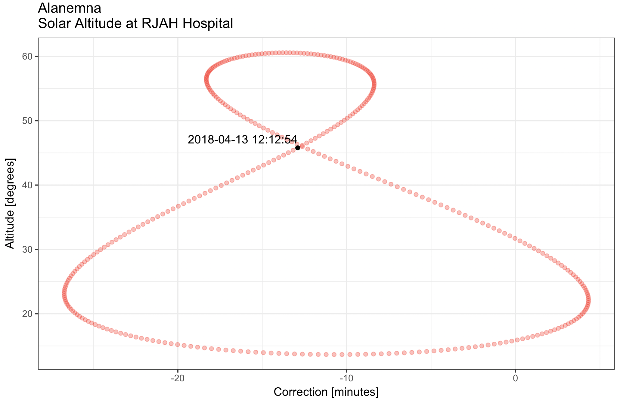
Rather than the solar declination, plot the solar altitude of the location (RJAH Hospital) on the y-axis and indicate the current day with the timing of solar noon:

dev.new()
solar_time %>%
ggplot(aes(x = total_correction / 60, y = altitude)) + # correction in mintues
geom_point(colour = “red”, alpha = 0.3) +
scale_x_continuous(“Correction [minutes]”) +
scale_y_continuous(“Altitude [degrees]”) +
ggtitle(“Alanemna\nSolar Altitude at RJAH Hospital”) +
geom_text(data = subset(solar_time, solar_time$day == yday(now(tzone = “GMT”))), aes(x = total_correction / 60, y = altitude, label = noon_apparent), hjust = 1, vjust = – 0.5) +
geom_point(data = subset(solar_time, solar_time$day == yday(now(tzone = “GMT”))), aes(x = total_correction / 60, y = altitude), colour = “black”) +
theme_bw()

To show the timings of the different twilights (civil, nautical and astronomical):

dev.new()
solar_time %>%
ggplot() +
geom_line(aes(x = day, y = (sun_rise – start)), colour = “red”) +
geom_line(aes(x = day, y = (sun_set – start)), colour = “orange”) +
# geom_line(aes(x = day, y = day_length), colour = ‘darkgreen’) +
geom_line(aes(x = day, y = (astro_rise – start) / 60), colour = “darkblue”) + # gives difference in minutes
geom_line(aes(x = day, y = (astro_set – start)), colour = “darkblue”) +
geom_line(aes(x = day, y = (nautical_rise – start)), colour = “blue”) +
geom_line(aes(x = day, y = (nautical_set – start)), colour = “blue”) +
geom_line(aes(x = day, y = (civil_rise – start)), colour = “steelblue”) +
geom_line(aes(x = day, y = (civil_set – start)), colour = “steelblue”) +
# add longest / shortest day earliest / latest sunrise / sunset
geom_vline(xintercept = longest_day$day, colour = “darkgreen”) +
geom_vline(xintercept = shortest_day$day, colour = “darkgreen”) +
geom_vline(xintercept = earliest_sun_rise$day, colour = “red”, linetype = 2) +
geom_vline(xintercept = latest_sun_rise$day, colour = “red”, linetype = 2) +
geom_vline(xintercept = earliest_sun_set$day, colour = “orange”, linetype = 2) +
geom_vline(xintercept = latest_sun_set$day, colour = “orange”, linetype = 2) +
# equinoxes
geom_vline(xintercept = 79, colour = “blue”, linetype = 3) +
geom_vline(xintercept = 266, colour = “blue”, linetype = 3) +
# astro twilight limits
geom_vline(xintercept = 132, colour = “darkblue”, linetype = 2) +
geom_vline(xintercept = 212, colour = “darkblue”, linetype = 2) +
scale_x_continuous(“Day Number”, limits = c(0, 375), breaks = c()) +
scale_x_continuous(“Day Number”, breaks = c(1, 79, 132, 212, 266, latest_sun_set$day, longest_day$day, earliest_sun_rise$day, latest_sun_rise$day, shortest_day$day, earliest_sun_set$day), limits = c(0, 375)) +
scale_y_continuous(“Hours after Midnight”) +
ggtitle(“Civil, Nautical and Astronomical Twilight”) +
theme_bw() +
theme(axis.text.x=element_text(angle = 90, hjust = 0, vjust = 0)) # after theme_bw call otherwise it doesnt’ work!
Scale for ‘x’ is already present. Adding another scale for ‘x’, which will replace the existing scale.

It is, of course, also possible to calculate the solar time from the computer time and estimate the timing of apparent solar noon:

###### calculate solar time based on computer time.
# use GMT, ignore British Summer Time
computer_time <- now(tzone = “GMT”)
year_day <- yday(computer_time)
correction_today <- equation_of_time(year_day) + longitude * 240
solar_time_today <- computer_time – correction_today
mean_solar_noon_today <- today() + dhours(12)
tz(mean_solar_noon_today) <- “GMT”
apparent_solar_noon_today <- mean_solar_noon_today – correction_today

computer_time
[1] “2018-04-13 15:37:41 GMT”
year_day
[1] 103
correction_today
[1] -774.042
solar_time_today
[1] “2018-04-13 15:50:35 GMT”
mean_solar_noon_today
[1] “2018-04-13 12:00:00 GMT”
apparent_solar_noon_today
[1] “2018-04-13 12:12:54 GMT”

Wickham H. tidyr: Easily Tidy Data with “spread()” and “gather()” Functions [Internet]. 2016. Available from: https://cran.r-project.org/web/packages/tidyr/index.html

Wickham H, Chang W. ggplot2: Create Elegant Data Visualisations Using the Grammar of Graphics [Internet]. Springer New York; 2016. Available from: http://cran.r-project.org/package=ggplot2

Grolemund G, Spinu V, WIckham H. lubridate: Make Dealing with Dates a Little Easier [Internet]. 2016. Available from: https://cran.r-project.org/web/packages/lubridate/index.html