Please make sure the necessary packages (seqinr 1 and Biostrings 2) are installed as described to allow analysis. Furthermore, the ggplot2 3 and reshape2 4 libraries should be loaded.
The genetic code for the lady’s slipper orchid (Cypripedium calceolus) can be downloaded. Select all the text (Ctrl-A), copy (Ctrl-C) and paste (Ctrl-V) it into a text editor. Save the file as ls_orchid.fasta (without a txt extension!) in the working directory (folder) of R.
Load the required library, import the fasta file as a list (orchid) and review the structure (str):
library(seqinr)
orchid <- read.fasta(file = “~/Desktop/ls_orchid.fasta”)
str(orchid)
List of 94
$ gi|2765658|emb|Z78533.1|CIZ78533:Class ‘SeqFastadna’ atomic [1:740] c g t a …
.. ..- attr(*, “name”)= chr “gi|2765658|emb|Z78533.1|CIZ78533″
.. ..- attr(*, “Annot”)= chr “>gi|2765658|emb|Z78533.1|CIZ78533 C.irapeanum 5.8S rRNA gene and ITS1 and ITS2 DNA”
…
…
.. ..- attr(*, “name”)= chr “gi|2765564|emb|Z78439.1|PBZ78439″
.. ..- attr(*, “Annot”)= chr “>gi|2765564|emb|Z78439.1|PBZ78439 P.barbatum 5.8S rRNA gene and ITS1 and ITS2 DNA”
The information is stored in a list. Every sequence can be viewed separately. To view the first sequence:
orchid[1]
$`gi|2765658|emb|Z78533.1|CIZ78533`
[1] “c” “g” “t” “a” “a” “c” “a” “a” “g” “g” “t” “t” “t” “c” “c” “g” “t” “a” “g” “g” “t” “g” “a”
– – –
[714] “a” “g” “g” “c” “g” “g” “g” “g” “g” “c” “a” “c” “c” “c” “g” “c” “t” “g” “a” “g” “t” “t” “t”
[737] “a” “c” “g” “c”
attr(,”name”)
[1] “gi|2765658|emb|Z78533.1|CIZ78533″
attr(,”Annot”)
[1] “>gi|2765658|emb|Z78533.1|CIZ78533 C.irapeanum 5.8S rRNA gene and ITS1 and ITS2 DNA”
attr(,”class”)
[1] “SeqFastadna”
and the last:
orchid[94]
$`gi|2765564|emb|Z78439.1|PBZ78439`
[1] “c” “a” “t” “t” “g” “t” “t” “g” “a” “g” “a” “t” “c” “a” “c” “a” “t” “a” “a” “t” “a” “a” “t”
– – –
[553] “a” “t” “t” “g” “t” “t” “g” “t” “g” “c” “a” “a” “a” “t” “g” “c” “c” “c” “c” “g” “g” “t” “t”
[576] “g” “g” “c” “c” “g” “t” “t” “t” “a” “g” “t” “t” “g” “g” “g” “c” “c”
attr(,”name”)
[1] “gi|2765564|emb|Z78439.1|PBZ78439″
attr(,”Annot”)
[1] “>gi|2765564|emb|Z78439.1|PBZ78439 P.barbatum 5.8S rRNA gene and ITS1 and ITS2 DNA”
attr(,”class”)
[1] “SeqFastadna”
To show the total number of sequences:
number_sequences <- length(orchid)
number_sequences
[1] 94
To show the length of the first and the last sequence:
length(orchid[[1]])
[1] 740
length(orchid[[number_sequences]])
[1] 592
To create a table of the nucleotides and calculate the GC (Guanine – Cytosine) content (more stable as three hydrogen bonds):
table <- table(orchid[[1]])
table
a c g t
144 200 241 155
str(table)
‘table’ int [1:4(1d)] 144 200 241 155
– attr(*, “dimnames”)=List of 1
..$ : chr [1:4] “a” “c” “g” “t”
table[1]
a
144
table[2]
c
200
table[3]
g
241
table[4]
t
155
# calculate the gc content:
gc_content <- (table[3] + table[2]) / sum(table)
gc_content
g
0.5959459
Or, the easy way:
GC(orchid[[1]])
[1] 0.5959459
So, almost 60%. It is also easy to count single nucleotides or combinations thereof:
count(orchid[[1]], 1)
a c g t
144 200 241 155
count(orchid[[1]], 2)
aa ac ag at ca cc cg ct ga gc gg gt ta tc tg tt
41 27 39 37 39 66 61 33 53 70 73 45 11 36 68 40
count(orchid[[1]], 3)
aaa aac aag aat aca acc acg act aga agc agg agt ata atc atg att caa cac cag cat cca ccc ccg cct
7 11 12 11 3 15 7 2 6 11 16 6 4 10 15 8 11 4 12 12 14 23 20 9
cga cgc cgg cgt cta ctc ctg ctt gaa gac gag gat gca gcc gcg gct gga ggc ggg ggt gta gtc gtg gtt
9 14 25 13 3 11 9 10 19 9 12 13 16 18 22 13 19 26 15 13 3 10 22 10
taa tac tag tat tca tcc tcg tct tga tgc tgg tgt tta ttc ttg ttt
4 3 3 1 6 10 11 9 19 19 17 13 1 5 22 12
# the output is a table object. So the extract is easy:
count(orchid[[1]], 1)[3]
g
241
# or better, refer by name:
count(orchid[[1]], 1)[“g”]
g
241
# similarly to count a specific triplets of nucleotides:
count(orchid[[1]], 3)[“att”]
att
8
Show the GC content for every sequence, reshape the data with reshape2 4 and plot with ggplot2 3:
# show sequence length and GC content in each sequence:
seq_lengths <- lapply(orchid, length)
seq_lengths_gc <- lapply(orchid, GC)
Reshape and plot the data:
gcs_plot <- melt(seq_lengths_gc)
lengths_plot <- melt(seq_lengths)
plot_data <- data.frame(length = lengths_plot, gc = gcs_plot)
ggplot(plot_data, aes(x = length.value, y = gc.value)) +
geom_point() +
theme_bw()

So the majority of sequences have a GC content of around 50%. There is however a group of longer sequences that have a GC content of more than 55%.
Sliding window plots are often used to show how the GC content varies along the sequence. Here, we create a sliding window plot of the longest (38th) sequence per 100 base pairs:
# sliding window plot to show GC content per 100 base pairs for sequence 38:
starts <- seq(1, length(orchid[[38]]) – 100, by = 100)
n <- length(starts) # how many chunks?
chunkGCs <- numeric(n) # null vector that has the same length as n
for (i in 1:n) {
chunk <- orchid[[38]][starts[i]:(starts[i] + 99)]
chunkGC <- GC(chunk)
chunkGCs[i] <- chunkGC
}
chunkGCs
[1] 0.43 0.60 0.55 0.45 0.59 0.57 0.49
plot_data_2 <- data.frame(location = starts, GC = chunkGCs)
dev.new()
ggplot(plot_data_2, aes(x = location, y = GC)) +
geom_line() +
theme_bw()

It is straight forward to get the single and triple letter amino acids coded for:
getTrans(orchid[[38]]) # this will give the standard one letter abbreviation
[1] “R” “N” “K” “V” “S” “V” “G” “E” “P” “P” “E” “G” “S” “L” “L” “R” “S” “H” “N” “N” “*” “S” “R”
– – –
[254] “T” “P” “G” “Q” “*” “A” “T” “R” “*” “V”
aaa(getTrans(orchid[[38]])) # will give the three letter abbreviation
[1] “Arg” “Asn” “Lys” “Val” “Ser” “Val” “Gly” “Glu” “Pro” “Pro” “Glu” “Gly” “Ser” “Leu” “Leu”
– —
[256] “Gly” “Gln” “Stp” “Ala” “Thr” “Arg” “Stp” “Val”
Dot plots are traditionally used to compare DNA sequences. The seqinr 1 package contains a function that creates a dot plot (called dotPlot). The number of nucleotides (wsize), step (wstep for overlap) and number of matches (nmatch) can be set. To compare single nucleotides of the 38th orchid sequence with itself:
dev.new()
dotPlot(orchid[[38]], orchid[[38]], wsize = 1, wstep = 1, nmatch = 1)
The diagonal line is uninterrupted, indicating the sequences are the same (obviously as the sequence was compared to itself).
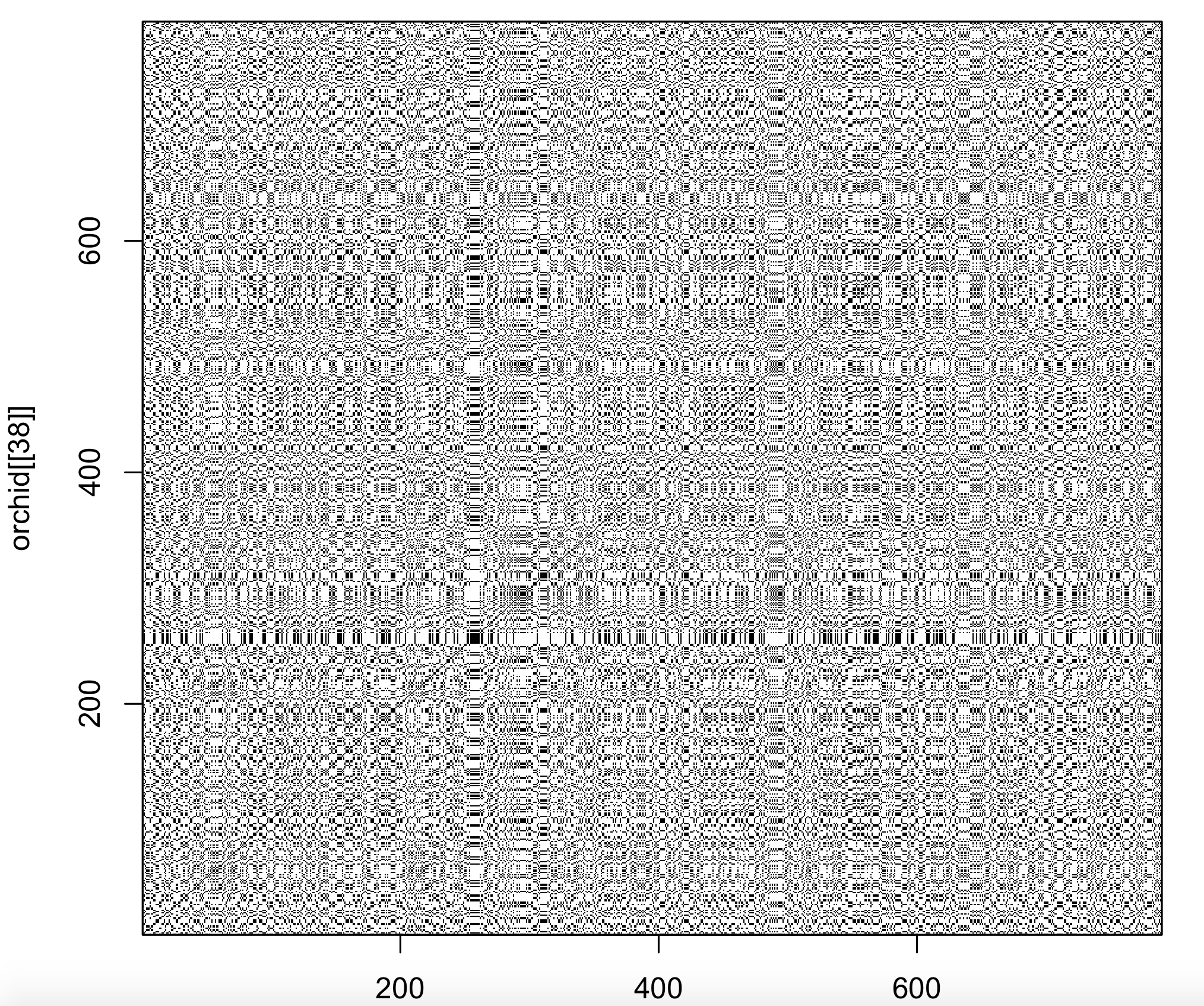
Or to compare triplets of nucleotides of the 38th orchid sequence with itself, specifying that all three nucleotides need to match (nmatch =3):
dev.new()
dotPlot(orchid[[38]], orchid[[38]], wsize = 3, wstep = 3, nmatch = 3)

The dot plot function included in the package is not very versatile. It would be better to plot with ggplot2 3. The main advantage of open source software is that the code of the functions is available to the user. The code of the dot plot was changed so that it returns a matrix (with sequence 1 as rows and sequence 2 as columns). The row names are the first sequence and the column names the second sequence. Copy and paste this function (called dot_plot_data) into the R console.
The new function (dot_plot_data) should now be available to R (it can also be viewed and downloaded from the download page). To access the function comparing three nucleotides and matching all three nucleotides takes the same format as the dotPlot function from the seqinr package 1 .
new_plot <- dot_plot_data(orchid[[38]], orchid[[38]], wsize = 3, wstep = 3, nmatch = 3)
Modification of dotPlot function in package seqinr.
The function returns a matrix for plotting.
Row names contain Sequence1, Col names Sequence2.
Use the reshape2 package to convert and plot with ggplot2 and geom_raster.
To show the structure and class of the returned object:
str(new_plot)
logi [1:263, 1:263] TRUE FALSE FALSE FALSE FALSE FALSE …
– attr(*, “dimnames”)=List of 2
..$ : chr [1:263] “cgt” “aac” “aag” “gtt” …
..$ : chr [1:263] “cgt” “aac” “aag” “gtt” …
class(new_plot)
[1] “matrix”
The data is now available as a matrix called new_plot. The row names are sequence 1 and the column names sequence 2. Unfortunately, ggplot2 3 can’t plot matrices directly. Consequently, the matrix need to be converted to a data frame suitable for plotting,
First, extract the row names and column names as vectors:
sequence_x <- rownames(new_plot)
sequence_y <- colnames(new_plot)
Secondly, remove the row and column names from the matrix (the names are not unique and otherwise ggplot2 3 will group by them):
rownames(new_plot) <- NULL
colnames(new_plot) <- NULL
Thirdly, use the reshape2 package 4 to reshape the data to allow plotting (the row and column numbers are unique, representing the number in the sequence):
new_plot_2 <- melt(new_plot)
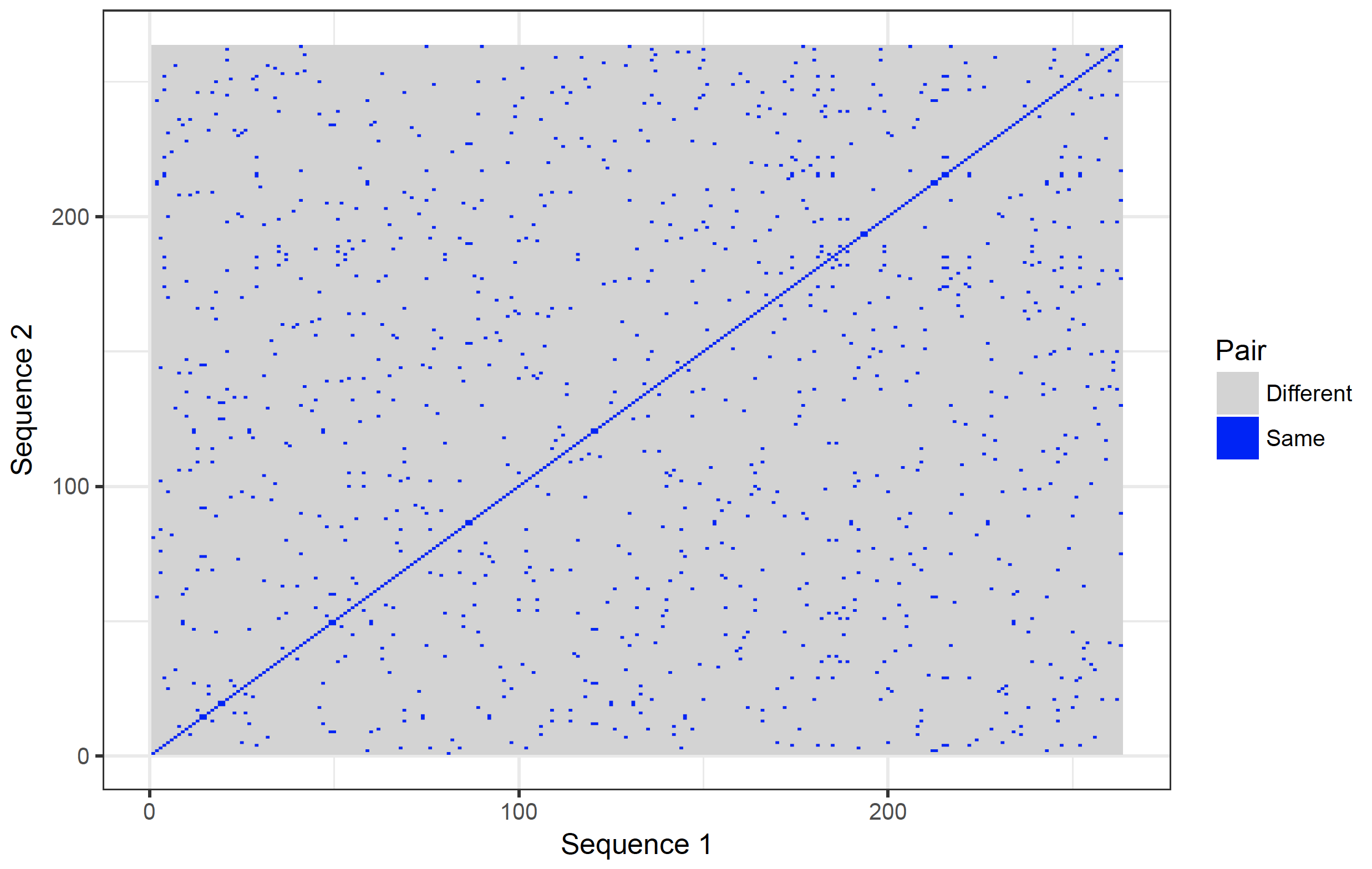
The data frame new_plot_2 has 3 columns (variables in tidy format). Var1 represents sequence 1 (x coordinate) and Var2 sequence 2 (y coordinate). The value variable contains the value stored in the matrix. To plot the data:
dot_plot <- ggplot(new_plot_2, aes(x = Var1, y = Var2, fill = value)) +
geom_raster() +
scale_fill_manual(values = c(“lightgray”, “blue”), name = “Pair”, labels = c(“Different”, “Same”)) +
scale_x_continuous(“Sequence 1″) +
scale_y_continuous(“Sequence 2″) +
theme_bw()
dev.new()
dot_plot
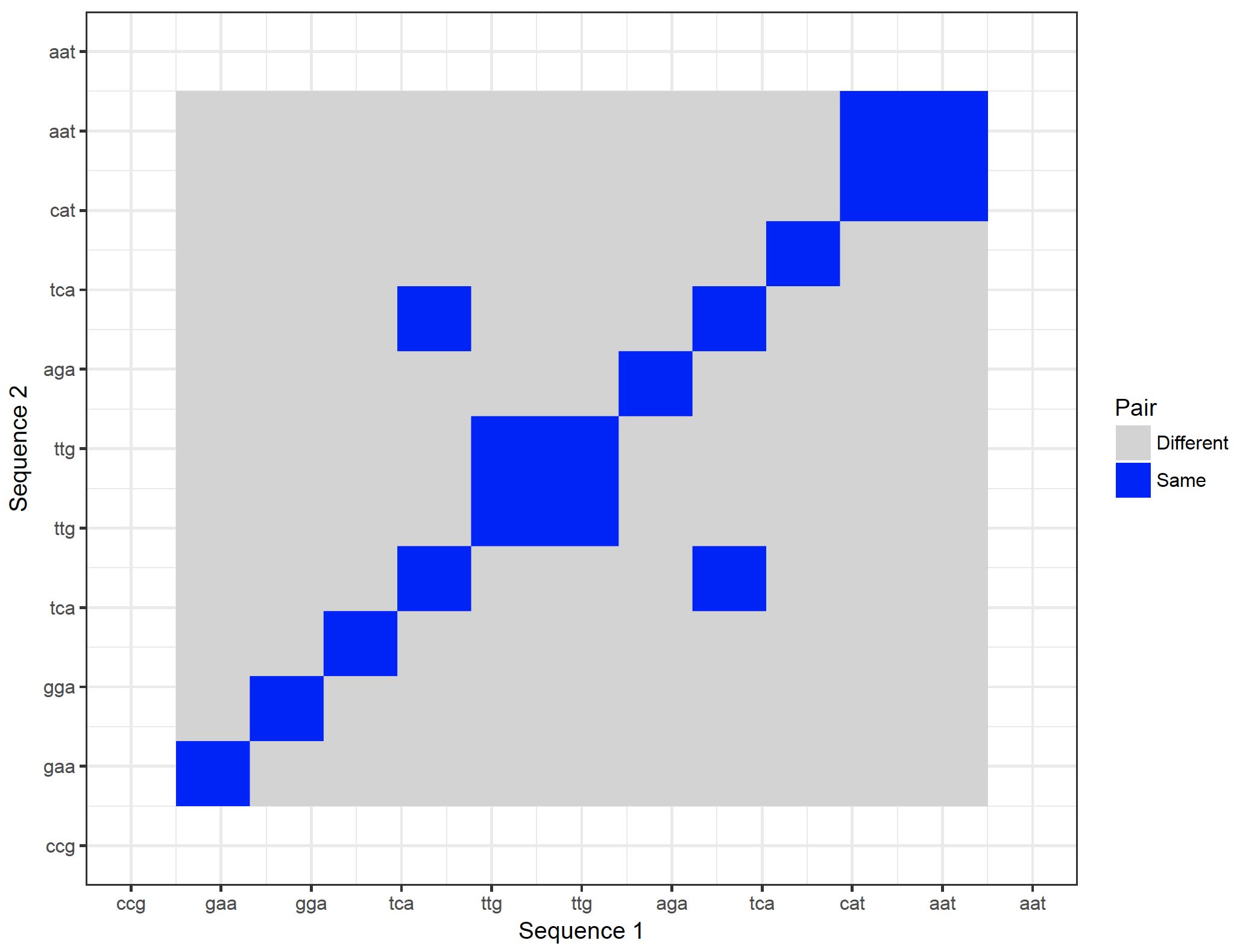
It is possible to show the nucleotides on the axes. However, they will become too crowded. It is possible to zoom in though:
dot_plot_2 <- ggplot(new_plot_2, aes(x = Var1, y = Var2, fill = value)) +
geom_raster() +
scale_fill_manual(values = c(“lightgray”, “blue”), name = “Pair”, labels = c(“Different”, “Same”)) +
scale_x_continuous(“Sequence 1″, breaks = 1: length(sequence_x), labels = sequence_x, limit = c(10,20)) +
scale_y_continuous(“Sequence 2″, breaks = 1: length(sequence_y), labels = sequence_y, limit = c(10,20)) +
theme_bw()
dev.new()
dot_plot_2
Warning message:
Removed 69048 rows containing missing values (geom_raster).
Finally, to save fasta files is straight forward. To save the orchid sequences to a fasta file (orchid_2) in the working directory:
write.fasta(names = c(1:94), sequences = orchid, file.out = “orchid_2.fasta”)