Please make sure the necessary packages (seqinr 1 and Biostrings 2) are installed as described to allow analysis. Furthermore, the ggplot2 3 and reshape2 4 libraries should be loaded.
In this section, the genetic sequence of the isocitrate dehydrogenase (IDH) 2 gene in humans is compared to that of orangutans. Mutations in the gene have been associated with Ollier’s disease and Maffucci syndrome in humans.
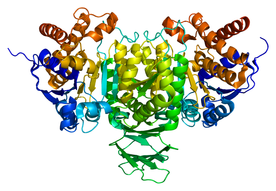
IDH is an enzyme that catalyses the oxidative decarboxylation of isocitrate. In humans, IDH has three forms: IDH1, IDH2 and IDH3. IDH3 catalyses the reaction with nicotinamide adenine dinucleotide (NAD+) as cofactor within the citric acid cycle, whilst IDH1 and IDH2 catalyse the reaction outside the citric acid cycle (with nicotinamide adenine dinucleotide phosphate (NADP+) as cofactor). Consequently, IDH1 and IDH2 are NADP+ dependent and IDH3 is NAD+ dependent.
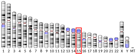
IDH2 is a mitochondrial enzyme,
encoded on chromosome 15 (in humans and orangutans):
The genetic code for human (homo sapiens) IDH2 can be downloaded here and the genetic code for an orangutan (pongo abelii) IDH2 here. Select all the text (Ctrl-A), copy (Ctrl-C) and paste (Ctrl-V) it into a text editor. Save the files as idh2_human.fasta and idh2_orangutan.fasta respectively (without a txt extension) in the working directory (folder) of R.
Load the files into R and examen the structure (str):
human <- read.fasta(file = “idh2_human.fasta”)
orangutan <- read.fasta(file = “idh2_orangutan.fasta”)
str(human)
List of 1
$ NG_023302.1:4923-23499:Class ‘SeqFastadna’ atomic [1:18577] t c c c …
.. ..- attr(*, “name”)= chr “NG_023302.1:4923-23499″
.. ..- attr(*, “Annot”)= chr “>NG_023302.1:4923-23499 Homo sapiens isocitrate dehydrogenase (NADP(+)) 2, mitochondrial (IDH2), RefSeqGene (LR”| __truncated__
str(orangutan)
List of 1
$ NC_036918.1:c70426964-70408539:Class ‘SeqFastadna’ atomic [1:18426] g c a a …
.. ..- attr(*, “name”)= chr “NC_036918.1:c70426964-70408539″
.. ..- attr(*, “Annot”)= chr “>NC_036918.1:c70426964-70408539 Pongo abelii isolate Susie chromosome 15, Susie_PABv2, whole genome shotgun sequence”
The sequences can be viewed by:
human[1]
$`NG_023302.1:4923-23499`
[1] “t” “c” “c” “c” “c” “g” “g” “c” “a” “a” “g” “g” “c” “c” “c” “a” “a” “t” “g” “g” “g” “g” “c”
– – – –
[18562] “a” “a” “a” “g” “c” “t” “c” “t” “t” “c” “a” “c” “a” “a” “a” “a”
attr(,”name”)
[1] “NG_023302.1:4923-23499″
attr(,”Annot”)
[1] “>NG_023302.1:4923-23499 Homo sapiens isocitrate dehydrogenase (NADP(+)) 2, mitochondrial (IDH2), RefSeqGene (LRG_611) on chromosome 15″
attr(,”class”)
[1] “SeqFastadna”
orangutan[1]
$`NC_036918.1:c70426964-70408539`
[1] “g” “c” “a” “a” “g” “g” “c” “c” “c” “a” “a” “t” “g” “g” “g” “g” “c” “g” “g” “c” “g” “g” “g”
– – – – –
[18401] “t” “a” “g” “c” “t” “a” “c” “t” “a” “a” “a” “a” “a” “g” “c” “t” “c” “t” “t” “c” “a” “c” “a”
[18424] “a” “a” “a”
attr(,”name”)
[1] “NC_036918.1:c70426964-70408539″
attr(,”Annot”)
[1] “>NC_036918.1:c70426964-70408539 Pongo abelii isolate Susie chromosome 15, Susie_PABv2, whole genome shotgun sequence”
attr(,”class”)
[1] “SeqFastadna”
The sequences are not of equal length:
length(human[[1]])
[1] 18577
length(orangutan[[1]])
[1] 18426
G-C bonds are more stable as they contain 3 hydrogen bonds whilst the A-T combination only has two. It is straight forward to create a table and calculate the G-C content:
human_table <- table(human[[1]])
human_table
a c g t
4244 4645 5144 4544
human_table[1]
a
4244
human_table[2]
c
4645
human_table[3]
g
5144
human_table[4]
t
4544
# calculate the g-c content:
gc_content_human <- (human_table[3] + human_table[2]) / sum(human_table)
gc_content_human
g
0.5269419
# or calculate GC content with the build in function:
GC(human[[1]])
[1] 0.5269419
orangutan_table <- table(orangutan[[1]])
orangutan_table
a c g t
4181 4591 5152 4502
orangutan_table[1]
a
4181
orangutan_table[2]
c
4591
orangutan_table[3]
g
5152
orangutan_table[4]
t
4502
# calculate the g-c content:
gc_content_orangutan <- (orangutan_table[3] + orangutan_table[2]) / sum(orangutan_table)
gc_content_orangutan
g
0.5287637
# or calculate GC content with the build in function:
GC(orangutan[[1]])
[1] 0.5287637
There is also a function to count individual nucleotides, or combinations of nucleotides:
count(human[[1]], 1) # for single nucleotides
a c g t
4244 4645 5144 4544
count(human[[1]], 2) # for pairs of nucleotides
aa ac ag at ca cc cg ct ga gc gg gt ta tc tg tt
1100 834 1479 830 1317 1486 393 1449 1152 1286 1690 1016 675 1039 1582 1248
count(human[[1]], 3) # for triplets of nucleotides (codons)
aaa aac aag aat aca acc acg act aga agc agg agt ata atc atg att caa cac cag cat cca ccc ccg cct
438 162 295 204 272 249 70 243 341 348 512 278 157 177 257 239 219 291 538 269 437 464 123 462
cga cgc cgg cgt cta ctc ctg ctt gaa gac gag gat gca gcc gcg gct gga ggc ggg ggt gta gtc gtg gtt
68 117 127 81 161 367 585 336 265 231 452 204 341 440 126 379 403 488 489 310 178 208 393 237
taa tac tag tat tca tcc tcg tct tga tgc tgg tgt tta ttc ttg ttt
178 150 194 153 267 333 74 365 340 333 562 347 179 286 347 436
# the output is a table object. So the extract is easy:
count(human[[1]], 1)[3] # using reference by place
g
5144
count(human[[1]], 1)[“g”] # using reference by name
g
5144
# similarly:
count(human[[1]], 3)[“att”]
att
239
count(orangutan[[1]], 1)
a c g t
4181 4591 5152 4502
count(orangutan[[1]], 2)
aa ac ag at ca cc cg ct ga gc gg gt ta tc tg tt
1076 834 1463 807 1284 1444 413 1450 1157 1277 1701 1017 664 1036 1574 1228
count(orangutan[[1]], 3)
aaa aac aag aat aca acc acg act aga agc agg agt ata atc atg att caa cac cag cat cca ccc ccg cct
422 176 280 197 267 244 70 253 344 348 497 274 144 179 246 238 216 278 533 257 413 443 134 454
cga cgc cgg cgt cta ctc ctg ctt gaa gac gag gat gca gcc gcg gct gga ggc ggg ggt gta gtc gtg gtt
67 127 140 79 169 376 591 314 263 230 453 211 339 430 129 379 402 477 509 313 175 206 408 228
taa tac tag tat tca tcc tcg tct tga tgc tgg tgt tta ttc ttg ttt
175 150 197 142 265 327 80 364 344 324 555 351 176 275 329 448
# the output is a table object. So the extract is easy:
count(orangutan[[1]], 1)[3] # reference by place
g
5152
count(orangutan[[1]], 1)[“g”] # reference by name
g
5152
# similarly:
count(orangutan[[1]], 3)[“att”]
att
238
So, the length of the sequences is similar (18577 in the human sequence and 18426 in the orangutan sequence), the combination att occurs 239 times in humans and 238 times in orangutans and the G-C content is also similar (52.7% in humans and 52.9% in orangutans).
To show the sequence lengths and G-C content in a bar chart (after reshaping with reshape2 4:
# show sequence length and GC content in each sequence (human and orangutan):
seq_lengths_human <- lapply(human, length)
seq_lengths_human_gc <- lapply(human, GC)
seq_lengths_orangutan <- lapply(orangutan, length)
seq_lengths_orangutan_gc <- lapply(orangutan, GC)
lengths_human_plot <- reshape2::melt(seq_lengths_human)
gcs_human_plot <- reshape2::melt(seq_lengths_human_gc)
lengths_orangutan_plot <- reshape2::melt(seq_lengths_orangutan)
gcs_orangutan_plot <- reshape2::melt(seq_lengths_orangutan_gc)
plot_data <- data.frame(human_length = lengths_human_plot, human_gc = gcs_human_plot, orangutan_length = lengths_orangutan_plot, orangutan_gc = gcs_orangutan_plot)
plot_data
human_length.value human_length.L1 human_gc.value human_gc.L1
1 18577 NG_023302.1:4923-23499 0.5269419 NG_023302.1:4923-23499
orangutan_length.value orangutan_length.L1 orangutan_gc.value
1 18426 NC_036918.1:c70426964-70408539 0.5287637
orangutan_gc.L1
1 NC_036918.1:c70426964-70408539
dev.new()
plot_data %>%
ggplot() +
geom_bar(aes(x = human_length.value, y = human_gc.value), stat = “identity”, colour = “black”, fill = “blue”, width = 10) +
geom_bar(aes(x = orangutan_length.value, y = orangutan_gc.value), stat = “identity”, colour = “black”, fill = “orange”, width = 10) +
scale_x_continuous(name = “Sequence Length”, limits = c(18400, 18600), breaks = c(18400, 18500, 18600, 18700)) +
scale_y_continuous(name = “G-C proportion”, limits = c(0.0, 0.6), breaks = c(0.0, 0.2, 0.4, 0.6)) +
theme_bw()

A sliding window plot is useful to compare the G-C content in different parts of the sequence. Here, we compare the G-C sequence in blocks of 1000 nucleotides and plot them with ggplot2 3:
# sliding window plot to show gc content per 1000 base pairs for sequences:
human_starts <- seq(1, length(human[[1]]) – 1000, by = 1000)
human_n <- length(human_starts) # how many chuncks?
human_chunkGCs <- numeric(human_n) # null vector that has the same length as n
for (i in 1:human_n) {
human_chunk <- human[[1]][human_starts[i]:(human_starts[i] + 999)]
human_chunkGC <- GC(human_chunk)
human_chunkGCs[i] <- human_chunkGC
}
human_chunkGCs
[1] 0.730 0.521 0.495 0.534 0.470 0.427 0.456 0.452 0.507 0.497 0.526 0.555 0.584 0.525 0.550
[16] 0.514 0.488 0.633
# and for orangutans:
orangutan_starts <- seq(1, length(orangutan[[1]]) – 1000, by = 1000)
orangutan_n <- length(orangutan_starts) # how many chuncks?
orangutan_chunkGCs <- numeric(orangutan_n) # null vector that has the same length as n
for (i in 1:orangutan_n) {
orangutan_chunk <- orangutan[[1]][orangutan_starts[i]:(orangutan_starts[i] + 999)]
orangutan_chunkGC <- GC(orangutan_chunk)
orangutan_chunkGCs[i] <- orangutan_chunkGC
}
orangutan_chunkGCs
[1] 0.719 0.523 0.499 0.528 0.463 0.435 0.464 0.451 0.498 0.510 0.536 0.556 0.585 0.534 0.553
[16] 0.528 0.494 0.638
dev.new()
ggplot() +
geom_line(aes(x = human_starts, y = human_chunkGCs), colour = “blue”) +
geom_line(aes(x = orangutan_starts, y = orangutan_chunkGCs), colour = “orange”) +
scale_x_continuous(name = “Sequence Position”, limits = c(0, 16000), breaks = c(5000, 10000, 15000)) +
scale_y_continuous(name = “GC proportion”, limits = c(0.0, 0.6), breaks = c(0.0, 0.2, 0.4, 0.6)) +
theme_bw()

To show the amino acids the nucleotides code for:
getTrans(human[[1]]) # this will give the standard one letter abbreviation
[1] “S” “P” “A” “R” “P” “N” “G” “A” “A” “G” “P” “A” “A” “P” “P” “R” “W” “C” “P” “R” “G” “Q” “R”
– – – –
[6188] “K” “A” “L” “H” “K”
aaa(getTrans(human[[1]])) # will give the three letter abbreviation
[1] “Ser” “Pro” “Ala” “Arg” “Pro” “Asn” “Gly” “Ala” “Ala” “Gly” “Pro” “Ala” “Ala” “Pro” “Pro”
– – – –
[6181] “Gly” “Ala” “Ile” “Phe” “Ser” “Tyr” “Stp” “Lys” “Ala” “Leu” “His” “Lys”
getTrans(orangutan[[1]]) # this will give the standard one letter abbreviation
[1] “A” “R” “P” “N” “G” “A” “A” “G” “P” “A” “A” “P” “P” “R” “W” “C” “P” “R” “G” “P” “R” “P” “P”
– – – –
[6142] “K”
aaa(getTrans(orangutan[[1]])) # will give the three letter abbreviation
[1] “Ala” “Arg” “Pro” “Asn” “Gly” “Ala” “Ala” “Gly” “Pro” “Ala” “Ala” “Pro” “Pro” “Arg” “Trp”
– – – – –
[6136] “Thr” “Lys” “Lys” “Leu” “Phe” “Thr” “Lys”
Traditionally, dot plots are used to compare DNA sequences. The seqinr package 1 does include a function to create dot plots. The number of nucleotides (wsize), step (wstep for overlap) and number of matches (nmatch) can be set. To compare chunks of 9 nucleotides, without overlap, in the DNA sequences of the IDH2 gene in humans and orangutans:
dotPlot(human[[1]], orangutan[[1]], wsize = 9, wstep = 9, nmatch = 9, col = c(“white”, “black”), xlab = deparse(substitute(human[[1]])), ylab = deparse(substitute(orangutan[[1]])))
Depending on the computer, it can take some time for the comparison to be completed:

The plot produced by the standard plot is a little difficult to assess , but this will be addressed later. If the sequences were the same, there should be a diagonal line from the origin of the plot to the upper right corner (similar as seen in the dot plot here). There seems little resemblance. Why is this? The sequences are not of the same length and not aligned. To compare the sequences, it is necessary to align them first.
To compare sequences, first define a scoring matrix. Here a score of +2 is given for a match and a score of -1 for a mismatch:
sigma <- nucleotideSubstitutionMatrix(match = 2, mismatch = -1, baseOnly = TRUE)
sigma # Print out the matrix
A C G T
A 2 -1 -1 -1
C -1 2 -1 -1
G -1 -1 2 -1
T -1 -1 -1 2
It is also required to convert the sequences to a string:
human_string <- getSequence(human[[1]], as.string = TRUE)
orangutan_string <- getSequence(orangutan[[1]], as.string = TRUE)
human_string <- toupper(human_string[[1]]) # convert to upper case
orangutan_string <- toupper(orangutan_string[[1]]) # convert to upper case
Now align the strings using the scoring matrix and setting gaps:
comparison <- pairwiseAlignment(human_string, orangutan_string, substitutionMatrix = sigma, gapOpening = -2, gapExtension = -8, scoreOnly = FALSE)
comparison
Global PairwiseAlignmentsSingleSubject (1 of 1)
pattern: [7] GCAAGGCCCAATGGGGCGGCAGGCCCGGCAGCCCCGCCCCGGTG…AACACATGGTGCCATATTTAGCTACTAAAAAGCTCTTCACAAAA
subject: [1] GCAAGGCCCAATGGGGCGGCGGGCCCGGCAGCCCCGCCCCGGTG…AACACATGGTGCCATATTTAGCTACTAAAAAGCTCTTCACAAAA
score: 32478
Considering there are 18577 base pairs and a score of 2 is given for a match, a score of 32478 is very convincing for similarity!
A function to review the aligned sequences is not part of the standard packages. However, Avril Coghlan 5 has published a function for this on her website. The function can be can be seen on this page and can be downloaded from here. To use the function, copy and paste the function into the R console and execute it. The function should now be available to R as “printPairwiseAlignment”. To show the alignment using the function:
> printPairwiseAlignment(comparison)
[1] “GCAAGGCCCAATGGGGCGGCAGGCCCGGCAGCCCCGCCCCGGTGGTGCCCGCGCGGCCAG 60″
[1] “GCAAGGCCCAATGGGGCGGCGGGCCCGGCAGCCCCGCCCCGGTGGTGTCCGCGCGGCCCG 60″
– – – –
[1] “CATGGTGCCATATTTAGCTACTAAAAAGCTCTTCACAAAA 18591″
[1] “CATGGTGCCATATTTAGCTACTAAAAAGCTCTTCACAAAA 18446″
This looks promising. To create a new dot plot with the aligned sequences:
# convert back to make dotplot as before
human_seq <- as.character(human_seq)
orangutan_seq <- as.character(orangutan_seq)
# convert to individual nucleotides rather than one long string:
human_seq <- getSequence(human_seq)
orangutan_seq <- getSequence(orangutan_seq)
dotPlot(human_seq, orangutan_seq, wsize = 9, wstep = 9, nmatch = 9, col = c(“white”, “black”))

This looks much better and the DNA sequences look very similar. However, the dot plot function included in the seqinr 1 package is not very versatile. It would be better to plot the comparison with ggplot2 3 .
The main advantage of open source software is that the code of functions is available to the user. The code of the dot plot was changed so that it returns a matrix (with sequence 1 as rows and sequence 2 as columns) rather than a plot. The row names are the first sequence and the column names the second sequence. Copy and paste this function (called dot_plot_data) into the R console and execute it.
The new function (dot_plot_data) should now be available to R (it can also be viewed and downloaded from the download page). To access the function comparing nine nucleotides and matching all nine nucleotides takes the same format as the dotPlot function from the seqinr package1:
new_plot <- dot_plot_data(human_seq, orangutan_seq, wsize = 9, wstep = 9, nmatch = 9)
To show the structure (str) and class of the returned object:
str(new_plot)
logi [1:2071, 1:2071] TRUE FALSE FALSE FALSE FALSE FALSE …
– attr(*, “dimnames”)=List of 2
..$ : chr [1:2071] “GCAAGGCCC” “AATGGGGCG” “GCAGGCCCG” “GCAGCCCCG” …
..$ : chr [1:2071] “GCAAGGCCC” “AATGGGGCG” “GCGGGCCCG” “GCAGCCCCG” …
class(new_plot)
[1] “matrix”
The data are now available as a matrix called new_plot. The row names are sequence 1 and the column names sequence 2. Unfortunately, ggplot2 3 can’t plot matrices directly. Consequently, the matrix need to be converted to a data frame suitable for plotting,
First, extract the row names and column names as vectors:
sequence_x <- rownames(new_plot)
sequence_y <- colnames(new_plot)
Secondly, remove the row and column names from the matrix (the names are not unique and otherwise ggplot2 3 will group by them):
rownames(new_plot) <- NULL
colnames(new_plot) <- NULL
Thirdly, use the reshape2 package 4 to reshape the data to allow plotting (the row and column numbers are unique, representing the number in the sequence):
new_plot_2 <- melt(new_plot)
The data frame new_plot_2 has 3 columns (variables in tidy format). Var1 represents sequence 1 (x coordinate) and Var2 sequence 2 (y coordinate). The value variable contains the value stored in the matrix. To plot the data:
dot_plot <- new_plot_2 %>%
ggplot(aes(x = Var1, y = Var2, fill = value)) +
geom_raster() +
scale_fill_manual(values = c(“lightgray”, “blue”), name = “Pair”, labels = c(“Different”, “Same”)) +
scale_x_continuous(“Human”) +
scale_y_continuous(“Orangutan”) +
theme_bw()
dev.new()
dot_plot

If the sequences would be indicated on the axes, the axes would become too crowded. However, the plot can be windowed (here between 10 and 20):
dot_plot_2 <- new_plot_2 %>%
ggplot(aes(x = Var1, y = Var2, fill = value)) +
geom_raster() +
scale_fill_manual(values = c(“lightgray”, “blue”), name = “Pair”, labels = c(“Different”, “Same”)) +
scale_x_continuous(“Human”, breaks = 1: length(sequence_x), labels = sequence_x, limit = c(10,20)) +
scale_y_continuous(“Orangutan”, breaks = 1: length(sequence_y), labels = sequence_y, limit = c(10,20)) +
theme_bw()
dev.new()
dot_plot_2
