Principle Component Analysis (PCA) is a linear transformation technique. It is an unsupervised machine learning method and consequently no classifier is necessary. To illustrate the method, R’s build in data set “iris” is used.
The build in iris data set contains the sepal and petal length and width of three different types of iris plants: Setosa, Versicolor and Virginica. Have a look at the iris data set:
head(iris)
Sepal.Length Sepal.Width Petal.Length Petal.Width Species
1 5.1 3.5 1.4 0.2 setosa
2 4.9 3.0 1.4 0.2 setosa
3 4.7 3.2 1.3 0.2 setosa
4 4.6 3.1 1.5 0.2 setosa
5 5.0 3.6 1.4 0.2 setosa
6 5.4 3.9 1.7 0.4 setosa
str(iris)
‘data.frame': 150 obs. of 5 variables:
$ Sepal.Length: num 5.1 4.9 4.7 4.6 5 5.4 4.6 5 4.4 4.9 …
$ Sepal.Width : num 3.5 3 3.2 3.1 3.6 3.9 3.4 3.4 2.9 3.1 …
$ Petal.Length: num 1.4 1.4 1.3 1.5 1.4 1.7 1.4 1.5 1.4 1.5 …
$ Petal.Width : num 0.2 0.2 0.2 0.2 0.2 0.4 0.3 0.2 0.2 0.1 …
$ Species : Factor w/ 3 levels “setosa”,”versicolor”,..: 1 1 1 1 1 1 1 1 1 1 …
A plot matrix of the first four numerical variables can be illustrative and is easily obtained:
plot(iris[,1:4])
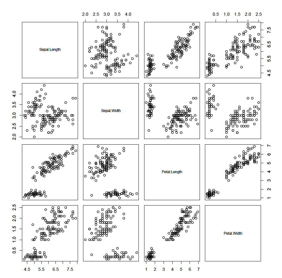
This illustrates that some variables are associated with each other. The aim of principle component analysis is to describe the data with linear combinations of the variables. Would it be possible to describe the data with less than 4 variables?? It is important to standardise the data first (mean = 0 and standard deviation = 1) as otherwise, the magnitude of a variable could have an influence. To standardise the four numerical variables (the categorical classifier is not needed as this is an unsupervised learning technique):
iris_standardised <- scale(iris[,1:4])
head(iris_standardised)
Sepal.Length Sepal.Width Petal.Length Petal.Width
[1,] -0.8976739 1.01560199 -1.335752 -1.311052
[2,] -1.1392005 -0.13153881 -1.335752 -1.311052
[3,] -1.3807271 0.32731751 -1.392399 -1.311052
[4,] -1.5014904 0.09788935 -1.279104 -1.311052
[5,] -1.0184372 1.24503015 -1.335752 -1.311052
[6,] -0.5353840 1.93331463 -1.165809 -1.048667
Next perform the principle component analysis on these standardised data and display a summary:
pca_iris <- prcomp(iris_standardised)
summary(pca_iris)
Importance of components:
PC1 PC2 PC3 PC4
Standard deviation 1.7084 0.9560 0.38309 0.14393
Proportion of Variance 0.7296 0.2285 0.03669 0.00518
Cumulative Proportion 0.7296 0.9581 0.99482 1.00000
The summary shows that the first principle component explains 73% of the variance, the second 96% and the third 99%. All variance is explained by all four components. To check this, sum the variances of each component (the standard deviation is stored in pca_iris$sdev):
pca_iris$sdev
[1] 1.7083611 0.9560494 0.3830886 0.1439265
# all variance should add up to the number of variables
sum(pca_iris$sdev^2)
[1] 4
So, the sum of the variances is four, which is the number of variables in the data set. How many principle components should be used to describe the data set? One component explains only 73% of the variance. Two components seems reasonable, but should be quantified. First draw a sreeplot:
screeplot(pca_iris, type = ‘lines’)
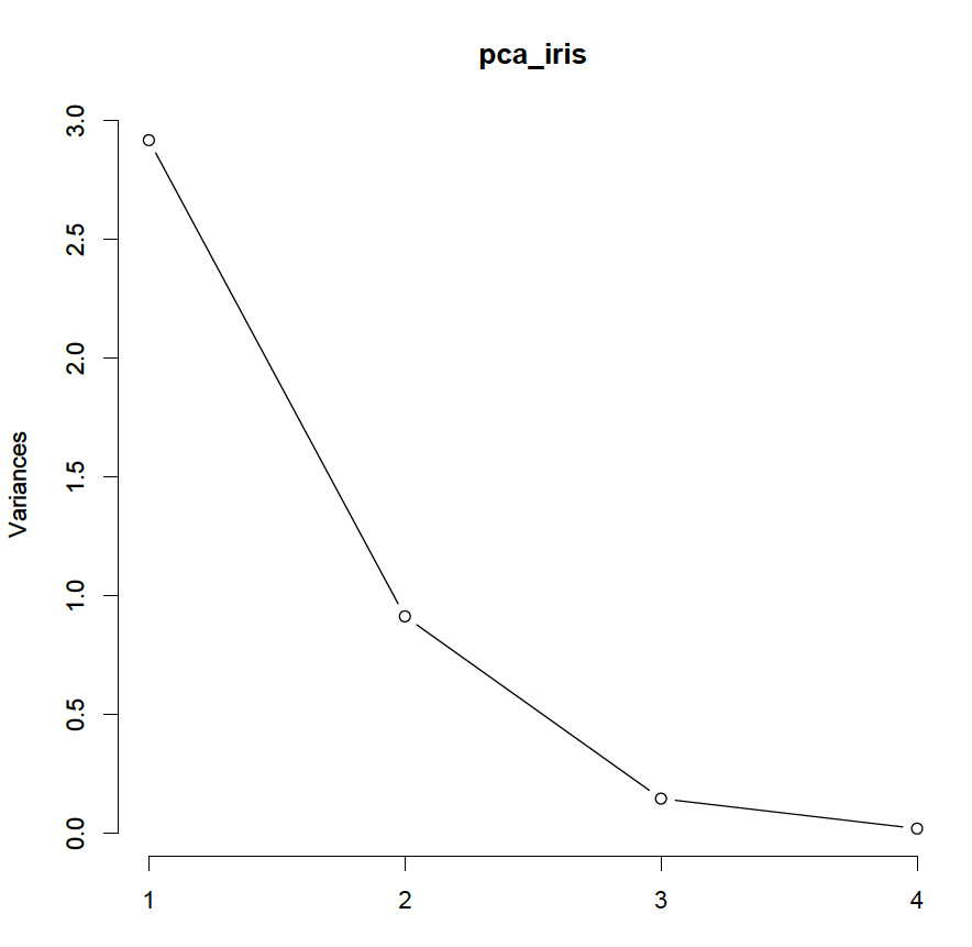 The elbow of the plot is at 3 principle components, so it is reasonable to maintain 2 principle components. Furthermore, according to Kaiser’s criterium, the variance of the last component on the standardised data should be less than 1; so again it is reasonable to use 2 principle components. Finally, to explain at least 80% of the variance, again 2 components are required.
The loadings of the first principle component can be obtained by:
pca_iris$rotation[,1]
Sepal.Length Sepal.Width Petal.Length Petal.Width
0.5210659 -0.2693474 0.5804131 0.5648565
and the second principle component by:
pca_iris$rotation[,2]
Sepal.Length Sepal.Width Petal.Length Petal.Width
-0.37741762 -0.92329566 -0.02449161 -0.06694199
The sum of all loadings should be one:
sum(pca_iris$rotation[,1]^2) # should be one
[1] 1
sum(pca_iris$rotation[,2]^2) # should be one
[1] 1
Looking at the loadings, the first principle component can be regarded as a contrast between sepal width and the other three variables (sepal length, petal width and petal length). The second principle component takes sepal width and length into account, but not petal length or width.
The first principle component can be plotted versus the second principle component to illustrate how the principle components separate the data into clusters. Remember, no classifier has been used, but the clusters are compared with the classifier as an illustration how principle component analysis can aid to gain insight:
iris_pca_df <- data.frame(first = pca_iris$x[,1], second = pca_iris$x[,2], species = iris$Species)
library(ggplot2)
ggplot(iris_pca_df, aes(x = first, y = second, colour = species)) +
geom_point() +
theme_bw() +
ggtitle(“Principle Component Analysis”) +
scale_x_continuous(“First Principle Component”) + scale_y_continuous(“Second Principle Component”)
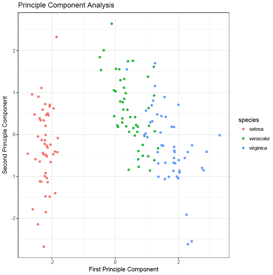
As can be seen the first principle component is good in separating Setosa species from the other two and to a lesser extend in separating Versicolar and Virginica species. The second principle component helps to separate Versicolar and Virginica species.