The ggplot2 library 1 is very versatile and allows the creation of high quality plots. In this section, it is shown how to import a custom font (ie Google), setting a theme for all subsequent plots and define custom colours / palettes.
Importing a custom font
Google has a large collection of fonts that is available for download. For example the Roboto fonts (standard, condensed, slab and monospaced) can be downloaded. Once downloaded, extract the zip file and save it to the fonts directory on you hard drive (Mac OSX: ~/Library/Fonts/ ). In Windows, right click on the ttf file and select install.
Once the font is installed on your system, R will need to know about it and import it to its database. This can be done with the extrafont package 2 available from the CRAN website. To install the package and load it:
install.packages(“extrafont”)
library(extrafont)
Registering fonts with R
To import all available fonts into R’s font database:
font_import()
but this may take a while.
To import a single font, specify the path to the font library (ie Mac OSX):
font_import(paths = “~/Library/Fonts”, pattern = “Roboto”)
To show the available / installed fonts:
fonttable()
Setting a custom theme
The ggplot2 library allows customisation of themes to create plots with similar layout. To define a custom theme (paul_theme):
library(ggplot2)
paul_theme <- function(base_size = 14, base_family = “Roboto”){
theme_minimal(base_size = base_size, base_family = base_family) +
theme(
axis.text = element_text(size=8),
axis.text.x = element_text(angle = 0, vjust = 0.5, hjust = 0.5),
axis.title = element_text(size =8),
panel.grid.major = element_line(color = “gray”),
panel.grid.minor = element_blank(),
panel.background = element_rect(fill = “#ffffff”),
strip.background = element_rect(fill = “black”, color = “black”, size =0.5),
strip.text = element_text(face = “bold”, size = 8, color = “white”),
legend.position = “bottom”,
legend.justification = “center”,
legend.background = element_blank(),
panel.border = element_rect(color = “grey5″, fill = NA, size = 0.5)
)
}
theme_set(paul_theme())
Defining colours
Once a plot has been created, it is straight forward to change a palette, by using the scale_color_brewer() function:
library(ggplot2)
data(mpg)
mpg
# A tibble: 234 x 11
manufacturer model displ year cyl trans drv cty hwy fl class
<chr> <chr> <dbl> <int> <int> <chr> <chr> <int> <int> <chr> <chr>
1 audi a4 1.8 1999 4 auto(l5) f 18 29 p compact
2 audi a4 1.8 1999 4 manual(m5) f 21 29 p compact
3 audi a4 2.0 2008 4 manual(m6) f 20 31 p compact
4 audi a4 2.0 2008 4 auto(av) f 21 30 p compact
5 audi a4 2.8 1999 6 auto(l5) f 16 26 p compact
6 audi a4 2.8 1999 6 manual(m5) f 18 26 p compact
7 audi a4 3.1 2008 6 auto(av) f 18 27 p compact
8 audi a4 quattro 1.8 1999 4 manual(m5) 4 18 26 p compact
9 audi a4 quattro 1.8 1999 4 auto(l5) 4 16 25 p compact
10 audi a4 quattro 2.0 2008 4 manual(m6) 4 20 28 p compact
# … with 224 more rows
ggplot(mpg, aes(x = hwy, y = cty, colour = class)) + geom_point() + theme_bw() + scale_color_brewer(palette = “Set2″) + ggtitle(“Set 2″)

ggplot(mpg, aes(x = hwy, y = cty, colour = class)) + geom_point() + theme_bw() + scale_color_brewer(palette = “Spectral”) + ggtitle(“Spectral Set”)

ggplot(mpg, aes(x = hwy, y = cty, colour = class)) + geom_point() + theme_bw() + scale_color_brewer(palette = “Blues”) + ggtitle(“Blues”)

It is also possible to define your own palette using the choose_palette() function in the colorspace package 3. To create a palette and give it a name (paul_palette):
library(colorspace)
paul_palette <- choose_palette()
The use interface will allow the creation of a custom palette based on the type of data and a default colour scheme. The number of colours to be available in the palette can also be selected:
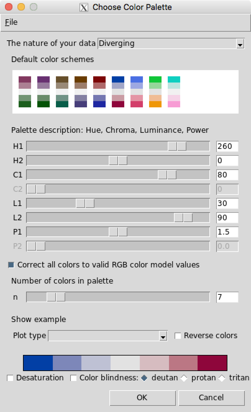
Once finished, select OK and the palette will be available as paul_palette. If 4 colours of the palette are required, use:
paul_palette(4)
[1] “#823960″ “#BD9AAA” “#91AA91″ “#1C5F1D”
You can also save a palette as an R file, by using the menu bar in colour picker. This will save a palette file to the working directory (ie pauls.R).
To load the palette, use source:
pauls <- source(“pauls.R”)
This is a function and to recreate the palette as pauls_palette:
pauls_palette <- pauls$value
pauls_palette(4)
[1] “#0FCFC0″ “#D5EAE7″ “#F3E1EB” “#F79CD4″
To show the palette create a vector of 10:
vector <- c(1:10)
vector
[1] 1 2 3 4 5 6 7 8 9 10
Create a breaks vector:
breaks <- c(0, vector)
breaks
[1] 0 1 2 3 4 5 6 7 8 9 10
A histogram of 5 colours:
hist(vector, breaks = breaks, col = pauls_palette(5))

A histogram of 10 colours:
hist(vector, breaks = breaks, col = pauls_palette(10))
