When reviewing papers, confidence intervals and p-values are often misinterpreted. In this short paper, the use of confidence intervals and p-values is illustrated with an example.
The table below shows a sample of 25 patients who had a Disability of the Arm, Shoulder and Hand (DASH) score 1;2 before surgery. A DASH score of 0% reflects no disability and normal function, whilst patients with a score of 100% are totally disabled.
Table 1:
| Case Number | DASH Score (%) |
|---|---|
| 1 | 95 |
| 2 | 100 |
| 3 | 71 |
| 4 | 92 |
| 5 | 55 |
| 6 | 100 |
| 7 | 98 |
| 8 | 39 |
| 9 | 92 |
| 10 | 74 |
| 11 | 73 |
| 12 | 90 |
| 13 | 33 |
| 14 | 81 |
| 15 | 76 |
| 16 | 44 |
| 17 | 96 |
| 18 | 47 |
| 19 | 47 |
| 20 | 86 |
| 21 | 96 |
| 22 | 39 |
| 23 | 89 |
| 24 | 94 |
| 25 | 69 |
Confidence intervals
Descriptive statistics are often used to summarise data with a measure of central tendency (mean, median and mode) and spread of the data (minimum value, maximum value, range, standard deviation and variance). Popular is Tukey’s five number summary 3 as shown in the table.
Table 2:
| Tukey's Five Numbers | Additional | ||
|---|---|---|---|
| Minimum | 33 | Mean | 75.0 |
| 1st Quartile | 55 | SD | 22.3 |
| Median | 81 | Variance | 497 |
| 3rd Quartile | 94 | Range | 67 |
| Maximum | 100 |
The table includes the minimum value, maximum value and median. The 1st and 3rd quartiles can be obtained by obtaining the median value of the data below and above median respectively. The median is the preferred measure of central tendency for data that have a skewed distribution as it is less influenced by outliers than the mean. However, the sample mean is often also obtained in medical literature.
The mean DASH score obtained from the sample would be different with a different sample of patients, and every different sample would have a different mean score. Of course, the mean DASH score in the population is not known, but may be estimated from the sample mean. But how do we estimate a confidence interval for the sample mean?
Method 1: Bootstrapping
One way of estimating the confidence interval for the sample mean is by a method called bootstrapping. In this method, the sample of 25 patients is re-sampled with replacement. Essentially the 25 DASH scores are put in a hat and a number is drawn blindly 25 times, whilst every time the drawn number is put back in the hat. In the new sample obtained, some values may be duplicate, but all the values in the re-sampled sample are present in the original sample (there are no new values added). This process can be repeated many times and multiple samples of 25 patients can be drawn from the original sample. Each sample is likely to be different and will have a different mean DASH score.
In theory, it would be possible for the re-sampled sample to have a mean DASH score of 100% (the DASH score of 100% from the original sample is drawn 25 times). Of course, this is very unlikely; in fact, the probability of this occurring would be (two patients had a DASH score of 100%):
However, the re-sampled sample can’t contain a DASH score of 0% as this score is not in the sample as shown in table 1.
Figure 1:
Figure 1 shows the mean DASH score of one million bootstrap samples taken from the sample in table 1. The 95% confidence interval of the mean DASH score can be obtained by finding the 2.5th and 97.5th percentile of that distribution. In this example, the bootstrap 95% confidence interval of the mean DASH score is between 66.2% and 83.3%. Therefore, the confidence interval reflects the re-sampled dataset and expresses the confidence in the mean as a value. The true mean in the population however, may well be outside this interval. Consequently, this is not a probability!
Figure 1 suggests the mean score is normally distributed. In fact, in can be shown that the distribution of the mean is always normal, even if the underlying distribution is not normal (central limit theory). The same is not true for other descriptive statistics such as the standard deviation (Figure 2). Figure 2 shows the bootstrapped distribution of the standard deviation to be left skew and not normal.
Figure 2:

Method 2: Equation
Given the original sample in table 1, the confidence interval of the mean DASH score can be calculated using the Standard Error or the Mean:
The 95% confidence interval of the mean DASH score is:
or between 66.3% and 83.7%. This is almost identical to the bootstrap sample obtained above.
Summary
The 95% confidence interval is NOT the probability of the true population mean being in this interval (this value is unknown). The true mean is either within the interval (probability is one) or outside the interval (probability is zero). The confidence interval merely reflects the confidence in the estimate. If the experiment is repeated 100 times, in a 95% confidence interval, the mean should be within that interval 95 times and be outside the interval 5 times (as shown in the bootstrap estimate). The smaller the sample standard deviation and the larger the number of observations in the sample, the narrower the confidence interval.
Testing for normality
A researcher may want to do further analysis using parametric statistics. This would require the data to be normally distributed. So how do we find out if the data are normally distributed?
Method 1: Kolmogorov–Smirnov test
To answer the question if the data in table 1 are normally distributed, a normality test, such as the Kolmogorov-Smirnov test could be performed. When this test is performed using R statistical software 3, a test statistic of D = 0.17447 is obtained, together with a p-value of 0.432. The Kolmogorov-Smirnov test is a test that compares two distributions. Here the sample distribution is compared to a normal distribution with the same mean and standard deviation as the sample. The null hypothesis is that the sample distribution doesn’t alter from the normal distribution. The p-value reflects the probability that the test statistic has a more extreme value than 0.17447. As the p-value is 0.432, it seems likely that the test statistic can obtain of more extreme value. Consequently, the null hypothesis is accepted (not rejected) and it could be concluded that the data are normally distributed.
However, is it reasonable to conclude that the data are normally distributed? Outcome scores, such as the DASH score, are often skewed and very unlikely to be normally distributed. Furthermore, the DASH score is obtained by adding scores to 30 different questions 1;2. Provided all questions are answered, the maximum score is 0%. If the person has mild difficulty in performing any one task, the total DASH score becomes 0.8%. Possible scores are 0%, 0.8%, 1.7%, 2.5%, 3.3% and so on. However, values in between these values are not possible. Consequently, the DASH score is not a continuous numerical variable, but discrete numerical.
Rather than just relying on a p-value, it would be better to have a more systematic approach in answering the question whether the data are normally distributed.
Method 2: Exploratory data analysis
As suggested by Tukey 1;2, it is often best to start with exploratory data analysis. The descriptive statistics obtained of the data are shown in table 2. The mean and median should be similar in normally distributed data, but they are quite different in this example (mean = 75% and median = 81%). Although the difference in these values are not incompatible with a normal distribution, they should at least instill some doubt.
Next, the data can be plotted. A histogram as shown in Figure 3:

clearly shows that the data are left skew and not normally distributed. In addition, a quantile-quantile plot can be used; where the quantiles of the sample are plotted against quantiles of a normal distribution.
Figure 4:
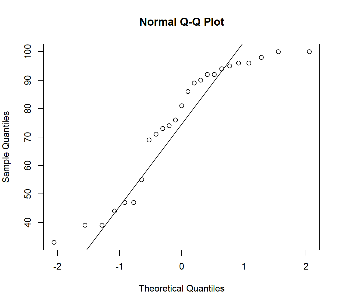
If normally distributed, the data should be on a straight line. This is clearly not the case, again suggesting a normal model for the data is inappropriate.
Method 3: W/S test
The W/S test is a simple and effective test for normality 4. The test statistic q (the standardised range) is the sample range divided by the sample standard deviation: 67 / 22.3 = 3 (Table 2). Therefore, the test statistic is 3. Statistical tables 4 show the critical value for the test statistic to be between 3.34 and 4.71 when p = 0.05. The test statistic is less than 3.34 (more extreme) and this is very unlikely under the null hypothesis of a normal distribution. Consequently, the null hypothesis is rejected and it is concluded that the data are not normally distributed.
Method 4: Shapiro-Wilk test
The Shapiro-Wilk test is a better normality test when the sample size is small. When obtained using R statistical software 4 a test statistic of W = 0.87457 is obtained with a p-value of 0.005. A more extreme value of the test statistic seems unlikely and the null hypothesis of the data being normally distributed is consequently rejected.
Method 5: Other tests
Many other tests for normality have been described, but outside the scope of this paper. It is not necessary to do all tests, but have a systematic and well-argued approach to the conclusions reached.
Summary
Despite the Kolmogorov-Smirnov test suggesting that a normal distribution may be a reasonable model for the sample data, further review and more in depth testing doesn’t confirm this. The Kolmogorov-Smirnov test is not ideal for small sample sizes; explaining the discrepancy (type 2 error).
Rather than depending on the results of one p-value, it is better to have a systematic approach and come to well-argued balanced conclusion.
It would be unusual for the DASH scores to be normally distributed and a left skew distribution seems a more appropriate description of the data. Here, the combination of common sense, descriptive statistics (difference between the mean and the median), a histogram, a quantile-quantile plot, the W/S test and the Shapiro-Wilk test provide strong evidence that the data do not conform a normal distribution.
Certain statistical tests (t-test and ANOVA) assume that the data are normally distributed and have equal variance. It is important to demonstrate that this assumption is reasonable when performing these tests. Although, ANOVA is known to be quite robust to violation of the normality rule, this should be considered and discussed in any paper.
P-values
In 2016, the American Statistical Association released a statement with six principles on statistical significance and p-values to improve the conduct and interpretation of quantitative science 5:
- P-values indicate how incompatible data are with a statistical model
- P-values do NOT measure the probability that the studied hypothesis is true
- Scientific conclusions should not be based only on whether a p-value is below a specified threshold
- Proper inference requires full reporting and transparency
- A p-value does NOT measure the size of an effect or the importance of a result
- On its own, a p-value does not provide a good measure of evidence regarding a model or hypothesis
One journal has now abandoned p-values in all publications 5. Authors can submit the results of statistical test in the manuscript; however, they will not be printed in the final publication. Although this may seem extreme, the editor took this step to encourage well-argued scientific methods rather than just relying on p-values.
Often researchers have large data sets with multiple variables that are subjected to many pair-wise comparisons. If 20 pair-wise statistical tests are performed; on average one test will be ‘significant’ at a p-value of 0.05 (type 1 error) just by chance. This is known as the multiple comparisons problem. To address the this, the p-value obtained can be corrected. There are several methods described, such as Bonferroni, Dunn and Holm 6. In the Bonferroni method, the p-value is corrected by dividing it by the number of statistical tests that are performed. If 20 statistical tests are performed, a p-value of 0.05 / 20 = 0.0025 will be regarded as ‘significant’. Not all statisticians agree with these p-value correction methods and p-value correction will increase the probability of false negatives (type 2 error) and reduced statistical power.
Although many journals will publish p-values of statistical tests, it is hoped authors are encouraged to use proper statistical inference with full reporting and transparency. When p-values are reported, exact p-values to three decimal places should be used. Only if the p-value is less than 0.1 %, the p-value should be reported as p < 0.001.
Learning points
Confidence intervals: A confidence interval of a value, reflects the confidence in the estimate. It is not a probability. When the value is repeatedly estimated, the 95% confidence interval contains the value 95% of the time.
P-values: The p-value represents the probability that the test statistic has a more extreme value than the one obtained. It is not the probability that the null hypothesis is true. On its own, the p-value is of little importance and should always be seen together with other supporting evidence.