Rather than using GGPLOT2 1, it is much easier to make swarm plots using the swarmplot package 2. The plot is similar to a strip plot with jitter, but the graphical presentation is more elegant.
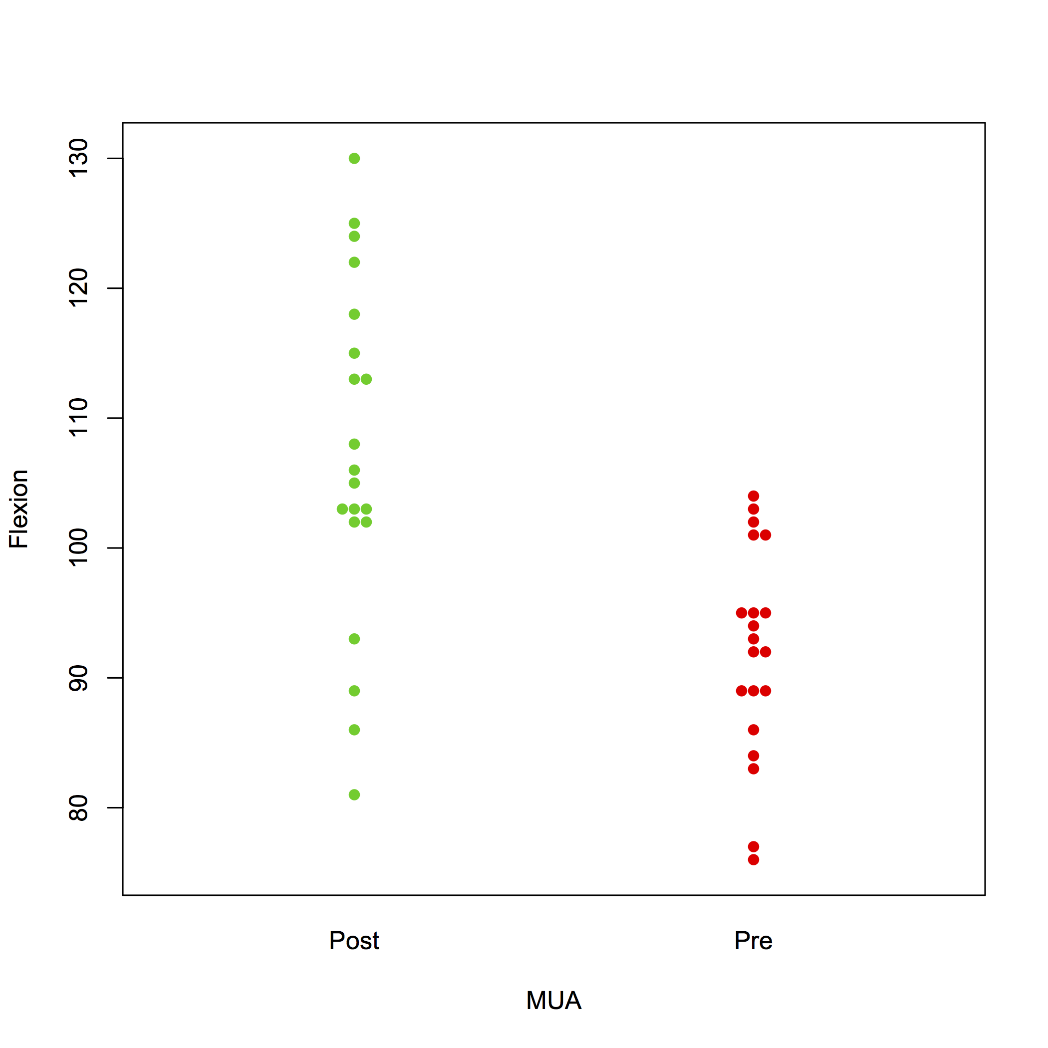
For this example, download and open the strip.rda dataset and open it in R / JGR. The data set contains the maximum flexion in 20 patients before and after a manipulation under anaesthesia. The data can be shown by:
strip
Flexion MUA
1 94 Pre
2 95 Pre
3 89 Pre
–
–
39 113 Post
40 86 Post
To create a swarm plot:
library(beeswarm)
beeswarm(Flexion ~ MUA, data = strip, col = 3:2, pch = 16 )
 For further option, please refer to the package manual 2.
A swarm plot can also be combined with a box plot:
beeswarm(Flexion ~ MUA, data = strip, col = 3:2, pch = 16, method = ‘center’ )
boxplot(Flexion ~ MUA, data = strip, add = TRUE)

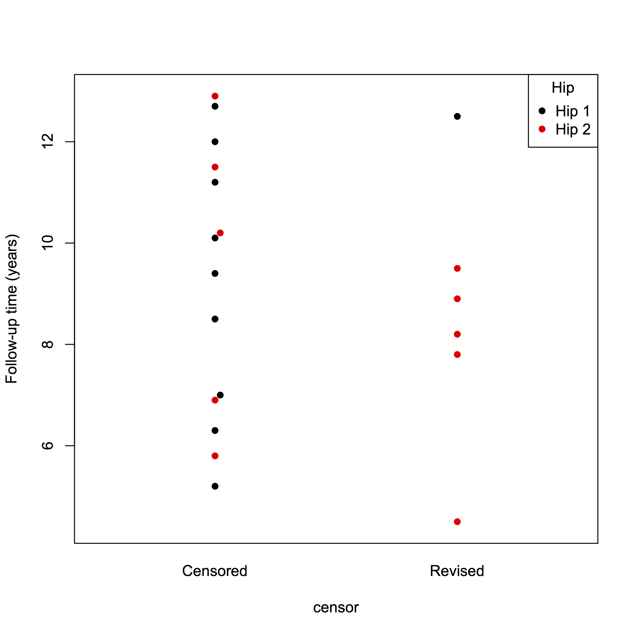
A swarm plot can also be used to visualise survival data as described in the survival chapter.
Download the plotsurvival.rda dataset for this example. The data frame is called plotsurvival and the variables are: number (patient number), fu (continuous; follow up time), group (categorical data; Hip 1 or Hip 2) and censor (binary outcome variable). To show the data:
plotsurvival
number fu group censor
1 1 5.2 Hip 1 0
2 2 6.3 Hip 1 0
3 3 7.0 Hip 1 0
–
18 18 10.2 Hip 2 0
19 19 11.5 Hip 2 0
20 20 12.9 Hip 2 0
To create a swarm plot of the data, with Hip 1 in black and Hip 2 in red:
library(beeswarm)
beeswarm(fu ~ censor, data = plotsurvival, pch = 16, pwcol = group, ylab = ‘Follow-up time (years)’, labels = c(‘Censored’, ‘Revised’))
legend(‘topright’, legend = levels(plotsurvival$group), title = ‘Hip’, pch = 16, col = 1:2)
 It is also possible to add a box plot.
library(beeswarm)
beeswarm(fu ~ censor, data = plotsurvival, pch = 16, pwcol = group, ylab = ‘Follow-up time (years)’, labels = c(‘Censored’, ‘Revised’))
boxplot(fu ~ censor, data = plotsurvival, add = TRUE)
legend(‘topright’, legend = levels(plotsurvival$group), title = ‘Hip’, pch = 16, col = 1:2)

For further options, please refer to the beeswarm 2 manual.