On this page, advanced concepts are discussed for the more experienced user. In particular, the manipulation of data and the assigning / arranging of new variables.
To rearrange / group data, it is useful to know several R operators / functions.
Helpful R Functions in Packages
Importing and Cleaning Data in R
R data manipulation functions examples:
To select a subset of data; for example select different observers (1 and 2) and create a new data frame with data of both observers in columns (the original data frame is called ‘results’ with as variables ‘observer’, ‘rotation’ and ‘outcome’):
observer1<-subset(results,observer==1,select=c(outcome, rotation))
names(observer1)[names(observer1)==”outcome”]<-‘outcome1′
names(observer1)[names(observer1)==”rotation”]<-‘rotation1′
observer2<-subset(results,observer==2,select=c(outcome,rotation))
names(observer2)[names(observer2)==”outcome”]<-‘outcome2′
names(observer2)[names(observer2)==”rotation”]<-‘rotation2′
observers<-cbind(observer1,observer2)
Some of these functions / operators are used in the examples below.
Printing percentages and currency signs:
To print percentages, use the sprintf function from R. For help on formatting, type ?sprintf in the console. A full description is outside the scope of this page. However, the first argument of the sprintf function should be within quotation marks (“). This argument starts with a % sign (to show a variable is coming), is followed by a full stop (to indicate the decimal point), followed by the number of decimal characters followed by an f (for floating point variable) and finally followed %% (the first percent sign is an ‘escape’ character as it would otherwise indicate a variable). The second argument of the function is the variable it should be applied to. Therefore, to print a percentage (%) sign behind a number:
a<-c(1,2,3,4,5,6,7,8,9)
a
[1] 1 2 3 4 5 6 7 8 9
b<-sprintf(“%.0f%%”,a)
b
[1] “1%” “2%” “3%” “4%” “5%” “6%” “7%” “8%” “9%”
Similarly, to print a % sign with two decimal places:
c<-sprintf(“%.2f%%”, a)
c
[1] “1.00%” “2.00%” “3.00%” “4.00%” “5.00%” “6.00%” “7.00%” “8.00%” “9.00%”
Finally, to print a £ sign (for example):
d<-sprintf(“£ %.2f”, a)
d
[1] “£ 1.00″ “£ 2.00″ “£ 3.00″ “£ 4.00″ “£ 5.00″ “£ 6.00″ “£ 7.00″ “£ 8.00″ “£ 9.00″
Manipulating dates:
Create a survival curve from dates; a data frame that contains the date of diagnosis and date of failure (example on how to convert dates to follow up time and how to create the censor variable; use survivaldates.rda with this example).
Revalue of map values (factors) with the plyr package 1 (for example month names from the first date of the month:
library(plyr)
month<-mapvalues(activity$ActivityMonth,from=c(’01/01/2014′,’01/02/2014′,’01/03/2014′,’01/04/2014′,’01/05/2014′,’01/06/2014′,’01/07/2014′,’01/08/2014′,’01/09/2014′,’01/10/2014′,’01/11/2014′,’01/12/2014′),to=c(‘Jan’,’Feb’,’Mar’,’Apr’,’May’,’Jun’,’Jul’,’Aug’,’Sep’,’Oct’,’Nov’,’Dec’))
Calculating the ‘day number’ of a date:
datum<-as.Date(as.character(’31/12/2000′),’%d/%m/%Y’)
datum
[1] “2000-12-31″
format(datum,format=’%j’)
[1] “366”
Convert incorrectly formatted data into appropriately declared variables that allow subsequent analysis:
It is a common error to group variables incorrectly and create a separate variable (column) for each group. However, variables should be in columns and the group is a separate variable. An example is show here.
Examples:
Please not that the functions also run from R (rather than JGR), but that the ggplot2 library 2 will have to be loaded separately.
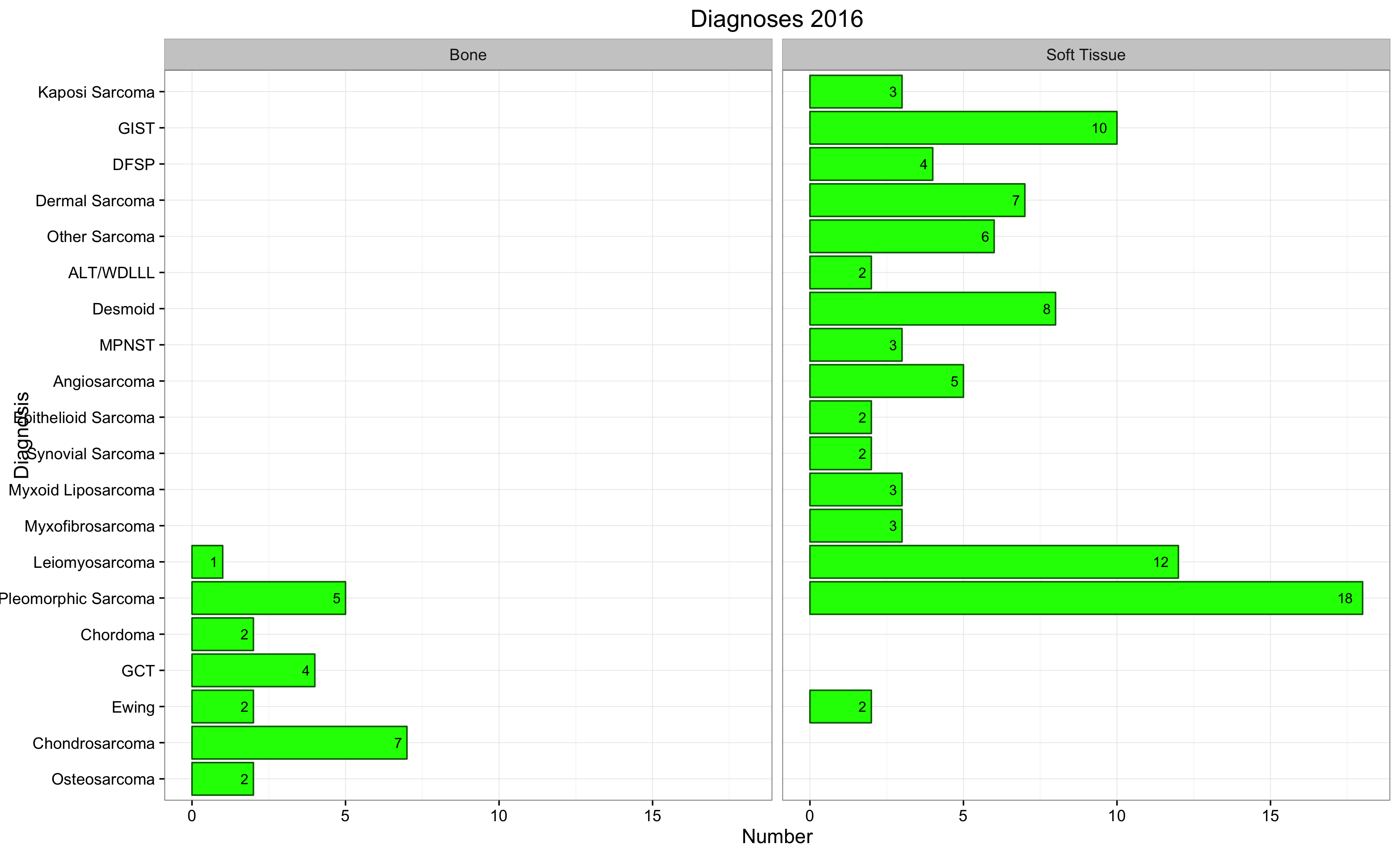
To create a faceted bar chart, load the Diag.rda data frame into JGR and run the create faceted bar chart function. This will create the following plot:
This example shows how to regroup data and create a plot on defined criteria.
To create a stacked and faceted bar plot, load the SpecGroup.rda data frame into JGR and run the stacked faceted bar plot 1 function. This will create the following plot:

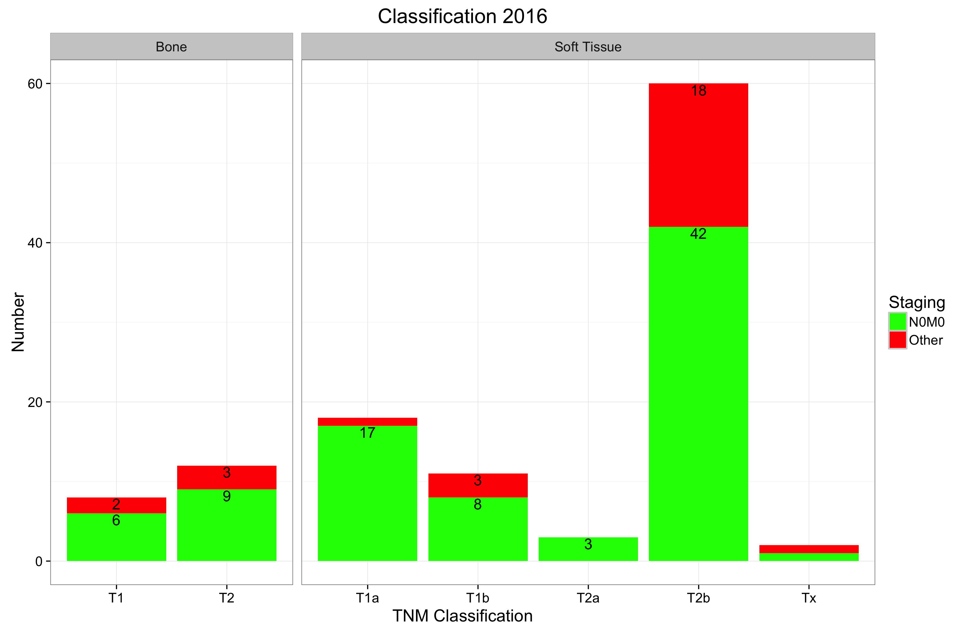
To create a stacked and faceted bar plot where the axes are ‘free’ and only labels that are greater than 1 are displayed; load the TNMstage.rdadata frame into JGR and run the stacked faceted bar plot 2 function. This will create the following plot: