Life table analysis is mostly obsolete in orthopaedics and Kaplan-Meier survival analysis is the preferred method as the exact failure time is usually known. Two variables are required:
- Follow up time (continuous variable)
- Censor (end point, nominal dichotomous variable (yes / no)).
An optional grouping variable to compare different groups:
- Grouping (nominal grouping variable)
Often the follow up time and censor need to be calculated from dates. In this respect the script survivaldates may be useful (this is an example script on how to convert dates to follow up time and how to create the censor variable; use survivaldates.rda with this example). Alternatively, a spreadsheet programs can be used to distract dates to calculates the follow up time.
The censor is a dichotomous variable as each patient can only in one of two states: uncensored or censored. Once the event of interest has occurred, the patient is uncensored. All other patients are censored. Patients can be censored due to :
- The event has not occurred before the end of the study
- The patient is lost to follow up during the study
- The patient withdraws from the study due to another reason (i.e. death)
So, before survival analysis can be performed, the data needs to be in an appropriate format. The data should be in a table with as many rows as there are patients. There should be at least two columns; a column for the continuous follow up variable and a column for the censor. A third grouping column is optional, but can be used to compare different groups of patients. Here, the plotsurvival.rda dataset is used with several methods on how to perform the analysis similar, but more in depth as described on the surival plot page. The methods described are:
- DeducerSurvival GUI
- Console method
- KM with Numbers function
- Prodlim package
DeducerSurvival GUI
Install the package survival 1 and DeducerSurvival with its dependencies as described.
DeducerSurvival (menu to create Kaplan-Meier survival curves)
It is however preferable to install the DeducerSurvival 2 function as a package from the CRAN website:
Please note there is a ‘bug’ in the program; the indication (colour) of groups in the legend and plot does not always coincide. Please check that the correct group is indicated in the legend. This will be corrected in a future release.
To perform survival analysis, choose ‘Survival’ and then ‘Kaplan Meier’ from the Deducer menu bar. In the dialogue box, choose ‘fu’ as ‘FollowUp’ and ‘censor’ as ‘Event':
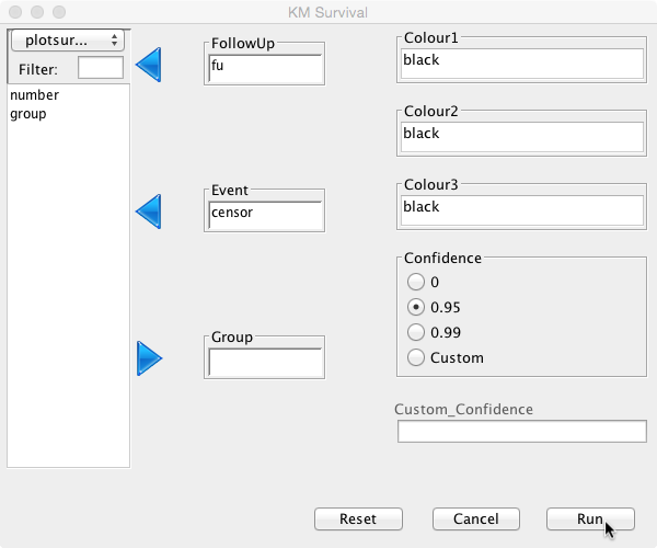
The default confidence interval is 95%, but this can be changed or switched off by selecting the appropriate radio button. A custom confidence level can also be set if so desired. Different colour options can be set for up to three curves. As no groups have been defined, only one colour is needed here. Initially, keep it at its default value ‘black’.
Click Run and the analysis will be performed:
mySurvival = with( plotsurvival , Surv( fu , censor ))
summary(mySurvival)
time status
Min. : 4.500 Min. :0.0
1st Qu.: 6.975 1st Qu.:0.0
Median : 9.150 Median :0.0
Mean : 9.055 Mean :0.3
3rd Qu.:11.275 3rd Qu.:1.0
Max. :12.900 Max. :1.0
mycurve=survfit(mySurvival~1,conf.int= 0.95 )
summary(mycurve)
Call: survfit(formula = mySurvival ~ 1, conf.int = 0.95)
time n.risk n.event survival std.err lower 95% CI upper 95% CI
4.5 20 1 0.950 0.0487 0.859 1.000
7.8 14 1 0.882 0.0795 0.739 1.000
8.2 13 1 0.814 0.0982 0.643 1.000
8.9 11 1 0.740 0.1138 0.548 1.000
9.5 9 1 0.658 0.1275 0.450 0.962
12.5 3 1 0.439 0.1982 0.181 1.000
plot(mycurve, col=c( ” black ” , ” black ” , ” black ” ))
title(main= “Kaplan Meier Curve” ,xlab= “Follow Up Duration” ,ylab= “Probability” )
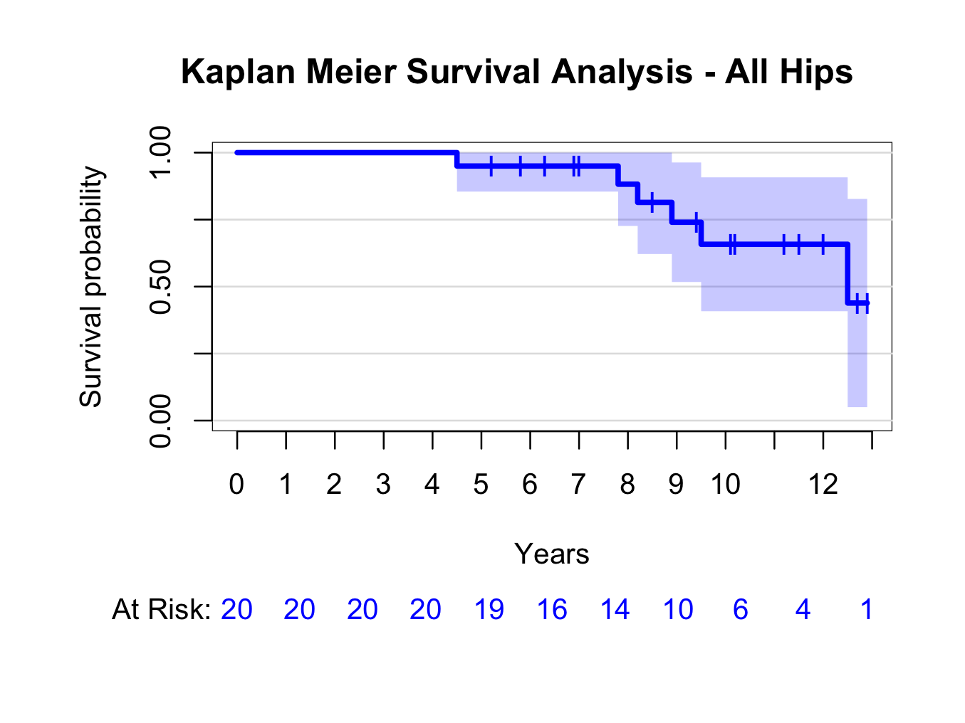
 The probability of survival can be read from the table and plot. The tick marks on the plot indicate patients that are censored (have no longer follow up time). The probability of survival of all hips is 43.9% at 12.5 years (the 10 year survival is 65.8%).
Groups
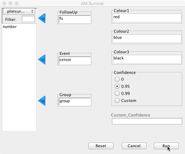
Different groups can be compared by selecting the ‘group’ variable as ‘Group’ in the dialogue box. Colours can be set to create a different colour for each group. Here there are two groups, ‘Hip 1′ and ‘Hip 2′. Select ‘red’ for ‘Colour1′ and ‘blue’ for ‘Colour2′ (but any other colour can be inserted; enter colors() in the console to obtain a full list of available colours):
mySurvival = with( plotsurvival , Surv( fu , censor ))
summary(mySurvival)
time status
Min. : 4.500 Min. :0.0
1st Qu.: 6.975 1st Qu.:0.0
Median : 9.150 Median :0.0
Mean : 9.055 Mean :0.3
3rd Qu.:11.275 3rd Qu.:1.0
Max. :12.900 Max. :1.0
mycurve=with( plotsurvival , survfit(mySurvival~ group ,conf.int= 0.95 ))
summary(mycurve)
Call: survfit(formula = mySurvival ~ group, conf.int = 0.95)
group=Hip 1
time n.risk n.event survival std.err lower 95% CI upper 95% CI
12.500 2.000 1.000 0.500 0.354 0.125 1.000
group=Hip 2
time n.risk n.event survival std.err lower 95% CI upper 95% CI
4.5 10 1 0.900 0.0949 0.732 1.00
7.8 7 1 0.771 0.1442 0.535 1.00
8.2 6 1 0.643 0.1679 0.385 1.00
8.9 5 1 0.514 0.1769 0.262 1.00
9.5 4 1 0.386 0.1732 0.160 0.93
plot(mycurve, col=c( ” red ” , ” blue ” , ” black ” ))
title(main= “Kaplan Meier Curve” ,xlab= “Follow Up Duration” ,ylab= “Probability” )
with( plotsurvival , legend(0,0.3,unique( group ),lty=c(1,1,1),col=c( ” red ” , ” blue ” , ” black ” )))
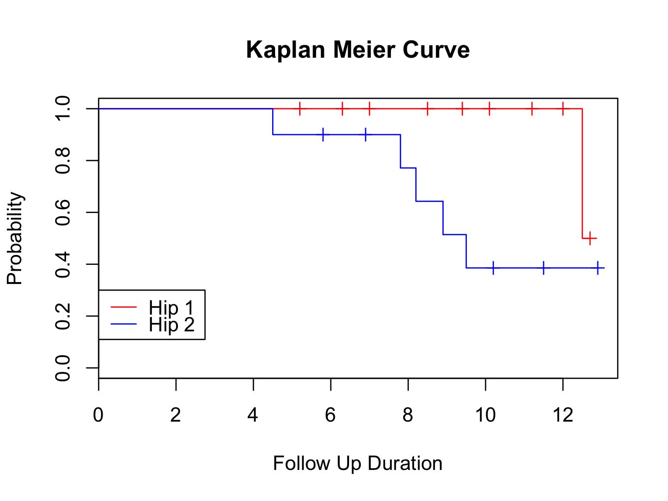
Please note that confidence levels are not routinely displayed for plots with multiple survival curves.
The survival curve suggests that Hip 1 performs better than Hip 2. However, at the tail end of the plot, the survival seems very similar. To decide if one group is better than the other, further analysis is required; either using a logrank test, Cox proportional hazards or parametric analysis (using a parametric distribution as model for the hazard). These methods are available in the DeducerSurvival menu under ‘Compare’.
Logrank test with DeducerSurvival
The logrank test is a non parametric test to compare two or more different survival curves. In essence, it is a Chi Square test on two or more curves. To perform the test between Hip 1 and Hip 2, select ‘Compare’ under the ‘Survival’ menu. Select ‘fu’ as ‘FollowUp’, ‘censor’ as ‘Event’ and ‘group’ as ‘Group':
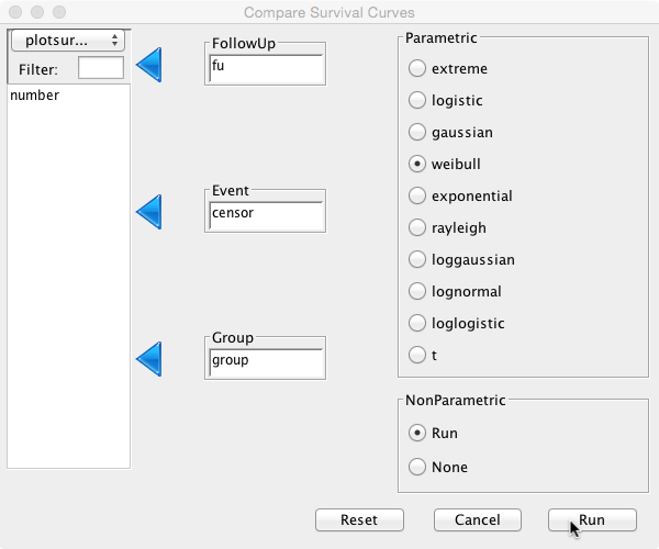
This will perform the logrank test as well as cox proportional hazards and parametric analysis (see below). With regards to the logrank test, the relevant output is:
mySurvival = with( plotsurvival , Surv( fu , censor ))
mylogrank=with( plotsurvival , survdiff(mySurvival~ group ))
mylogrank
Call:
survdiff(formula = mySurvival ~ group)
N Observed Expected (O-E)^2/E (O-E)^2/V
group=Hip 1 10 1 3.31 1.61 3.63
group=Hip 2 10 5 2.69 1.97 3.63
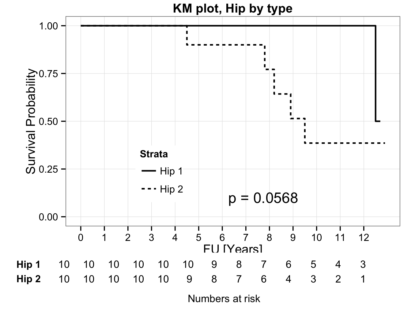
Chisq= 3.6 on 1 degrees of freedom, p= 0.0568
Therefore, no significant difference between the two hips has been demonstrated using the logrank test.
Cox proportional hazards with DeducerSurvival
The Cox proportional hazards test is a non parametric test that compares two or more survival curves. This test is commonly used in medicine and more is powerful than the logrank test.
As above, perform the analysis. With regards to the Cox proportional hazards, the relevant output is:
mycoxph=with( plotsurvival , coxph(mySurvival~ group ))
mycoxph
Call:
coxph(formula = mySurvival ~ group)
coef exp(coef) se(coef) z p
groupHip 2 1.84 6.28 1.10 1.67 0.095
Likelihood ratio test=3.84 on 1 df, p=0.05
n= 20, number of events= 6
So just significant!
Parametric analysis with DeducerSurvival
As above, the analysis is performed. The relevant parametric test can be selected. A full description is outside the scope of this book. Above, the ‘Weibull’ distribution was selected. A full description of this is outside the scope of this book. However, it assumes a hazard that increases over time (which seems appropriate for aseptic loosening). The relevant output from the analysis:
myparametric=with( plotsurvival , survreg(mySurvival~ group , dist = “weibull” ))
myparametric
Call:
survreg(formula = mySurvival ~ group, dist = “weibull”)
Coefficients:
(Intercept) groupHip 2
2.9364589 -0.5055782
Scale= 0.2617896
Loglik(model)= -20 Loglik(intercept only)= -22.2
Chisq= 4.31 on 1 degrees of freedom, p= 0.038
n= 20
Again showing statistical significance.
Console method
The survival package 1 should be installed and active.
library(survival)
To check the data frame is loaded:
plotsurvival
number fu group censor
1 1 5.2 Hip 1 0
2 2 6.3 Hip 1 0
3 3 7.0 Hip 1 0
4 4 8.5 Hip 1 0
5 5 9.4 Hip 1 0
6 6 10.1 Hip 1 0
7 7 11.2 Hip 1 0
8 8 12.0 Hip 1 0
9 9 12.5 Hip 1 1
10 10 12.7 Hip 1 0
11 11 4.5 Hip 2 1
12 12 5.8 Hip 2 0
13 13 6.9 Hip 2 0
14 14 7.8 Hip 2 1
15 15 8.2 Hip 2 1
16 16 8.9 Hip 2 1
17 17 9.5 Hip 2 1
18 18 10.2 Hip 2 0
19 19 11.5 Hip 2 0
20 20 12.9 Hip 2 0
To perform survival analysis for all hips together, first create a survival object and call this mysurvival:
mysurvival<-Surv(plotsurvival$fu,plotsurvival$censor)
To show the object:
mysurvival
[1] 5.2+ 6.3+ 7.0+ 8.5+ 9.4+ 10.1+ 11.2+ 12.0+ 12.5 12.7+ 4.5 5.8+ 6.9+ 7.8 8.2 8.9 9.5 10.2+ 11.5+ 12.9+
This shows the survival times of all patients. The follow up times followed by a ‘+’ are censored; the others have failed.
A summary of the object can be useful:
summary(mysurvival)
time status
Min. : 4.500 Min. :0.0
1st Qu.: 6.975 1st Qu.:0.0
Median : 9.150 Median :0.0
Mean : 9.055 Mean :0.3
3rd Qu.:11.275 3rd Qu.:1.0
Max. :12.900 Max. :1.0
So the shortest follow time is 4.5 years and the longest 12.9 years, with a median follow up time of 9.15 years.
Next, a Kaplan-Meier (product limit) survival curve, called mycurve, is fitted on the mysurvival object (without confidence levels):
mycurve<-survfit(mysurvival~1,conf.type=’none’)
Please note the tilde 1 (~1). This is a required grouping parameter. If there are no groups, it should be set to 1.
To show the survival estimate:
mycurve
Call: survfit(formula = mysurvival ~ 1, conf.type = “none”)
n events median
20.0 6.0 12.5
So, there are 20 patients of whom 6 failed. The median survival is the time it takes for the cumulative survival to become 50%. Here, the median survival is 12.5 years.
A more detailed summary can be useful:
summary(mycurve)
Call: survfit(formula = mysurvival ~ 1, conf.type = “none”)
time n.risk n.event survival std.err
4.5 20 1 0.950 0.0487
7.8 14 1 0.882 0.0795
8.2 13 1 0.814 0.0982
8.9 11 1 0.740 0.1138
9.5 9 1 0.658 0.1275
12.5 3 1 0.439 0.1982
It is easy to obtain a survival probability at a specified time. For example, the survival probability at 5 years is:
summary(mycurve,time=5)
Call: survfit(formula = mysurvival ~ 1, conf.type = “none”)
time n.risk n.event survival std.err
5 19 1 0.95 0.0487
or 48.7%; and the survival probability at 10 years is:
summary(mycurve,time=10)
Call: survfit(formula = mysurvival ~ 1, conf.type = “none”)
time n.risk n.event survival std.err
10 8 5 0.658 0.127
or 12.7%.
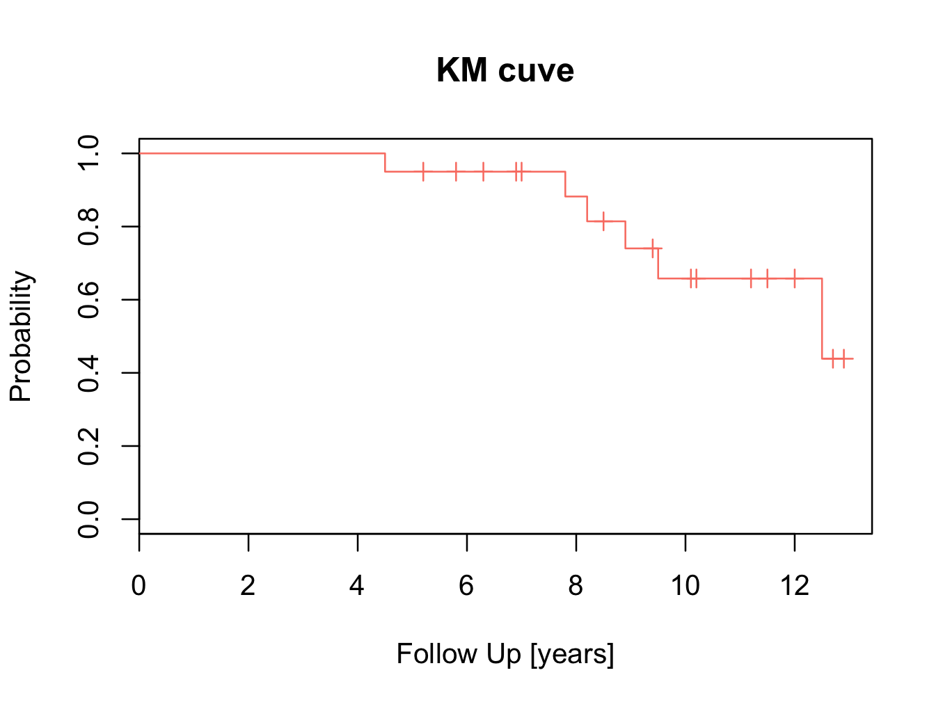
To show the survival curve:
plot(mycurve)
 and add axes labels:
title(main=’KM cuve’, xlab=’Follow Up [years]’,ylab=’Probability’)
 The censored patients are indicated by a tick mark on the survival curve. To create the plot in a different colour is easy:
plot(mycurve,col=’salmon’)
title(main=’KM cuve’, xlab=’Follow Up [years]’,ylab=’Probability’)
 For a full list of available colours:
colors()
Output omitted for brevity.
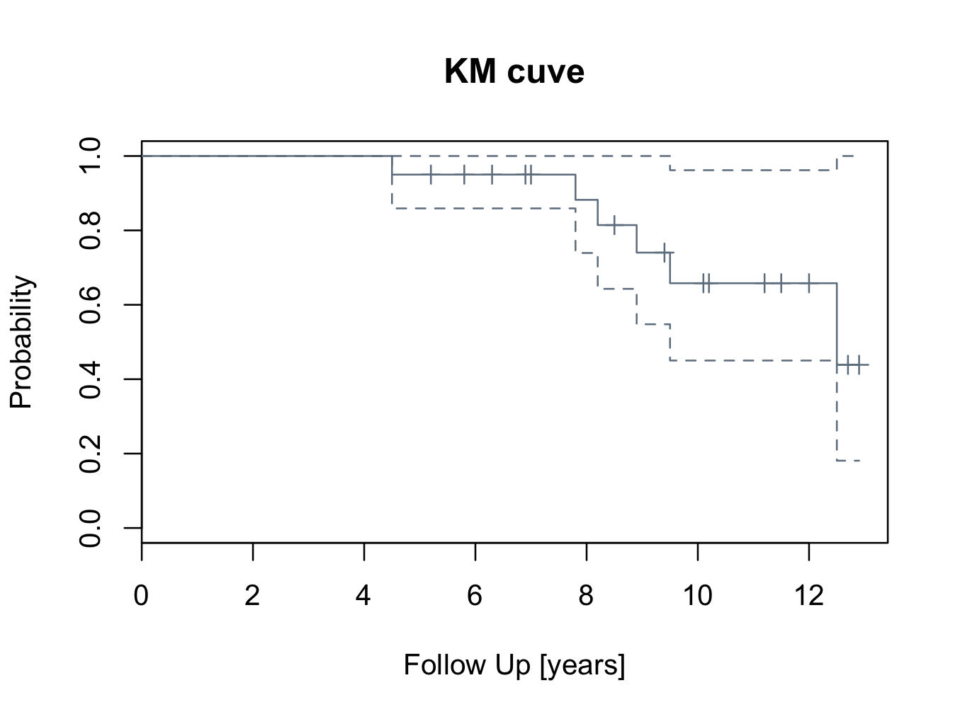
To add a confidence interval to the survival curve is also straight forward and should be included in the mycurve object:
mycurve<-survfit(mysurvival~1,conf.int=0.95)
summary(mycurve)
Call: survfit(formula = mysurvival ~ 1, conf.int = 0.95)
time n.risk n.event survival std.err lower 95% CI upper 95% CI
4.5 20 1 0.950 0.0487 0.859 1.000
7.8 14 1 0.882 0.0795 0.739 1.000
8.2 13 1 0.814 0.0982 0.643 1.000
8.9 11 1 0.740 0.1138 0.548 1.000
9.5 9 1 0.658 0.1275 0.450 0.962
12.5 3 1 0.439 0.1982 0.181 1.000
The confidence interval can be changed by altering the conf.int value.
To plot a ‘slategray’ curve with confidence intervals:
plot(mycurve,col=’slategray’)
title(main=’KM cuve’, xlab=’Follow Up [years]’,ylab=’Probability’)
 Groups
Create a survival object similar as to described above. However, in the Kaplan Meier estimate object, set the grouping variable after the tilde (~) sign (here the ‘group’ variable in the ‘plotsurvival’ data frame).
mysurvival<-Surv(plotsurvival$fu,plotsurvival$censor)
mysurvival
[1] 5.2+ 6.3+ 7.0+ 8.5+ 9.4+ 10.1+ 11.2+ 12.0+ 12.5 12.7+ 4.5 5.8+ 6.9+ 7.8 8.2 8.9 9.5 10.2+ 11.5+ 12.9+
mycurve=survfit(mysurvival~plotsurvival$group,conf.type=’none’)
mycurve
Call: survfit(formula = mysurvival ~ plotsurvival$group, conf.type = “none”)
n events median
plotsurvival$group=Hip 1 10 1 12.5
plotsurvival$group=Hip 2 10 5 9.5
summary(mycurve)
Call: survfit(formula = mysurvival ~ plotsurvival$group, conf.type = “none”)
plotsurvival$group=Hip 1
time n.risk n.event survival std.err
12.500 2.000 1.000 0.500 0.354
plotsurvival$group=Hip 2
time n.risk n.event survival std.err
4.5 10 1 0.900 0.0949
7.8 7 1 0.771 0.1442
8.2 6 1 0.643 0.1679
8.9 5 1 0.514 0.1769
9.5 4 1 0.386 0.1732
Now plot the curves with labels to the axes and a title:
plot(mycurve,col=c(‘wheat’,’green’))
title(main=’KM curve’,xlab=’FU [years]’, ylab=’Probability’)
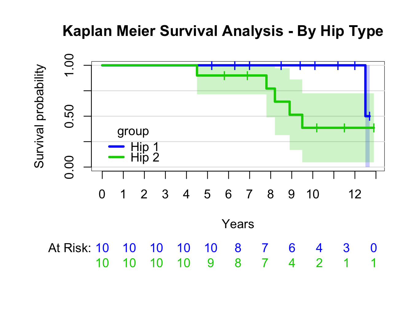
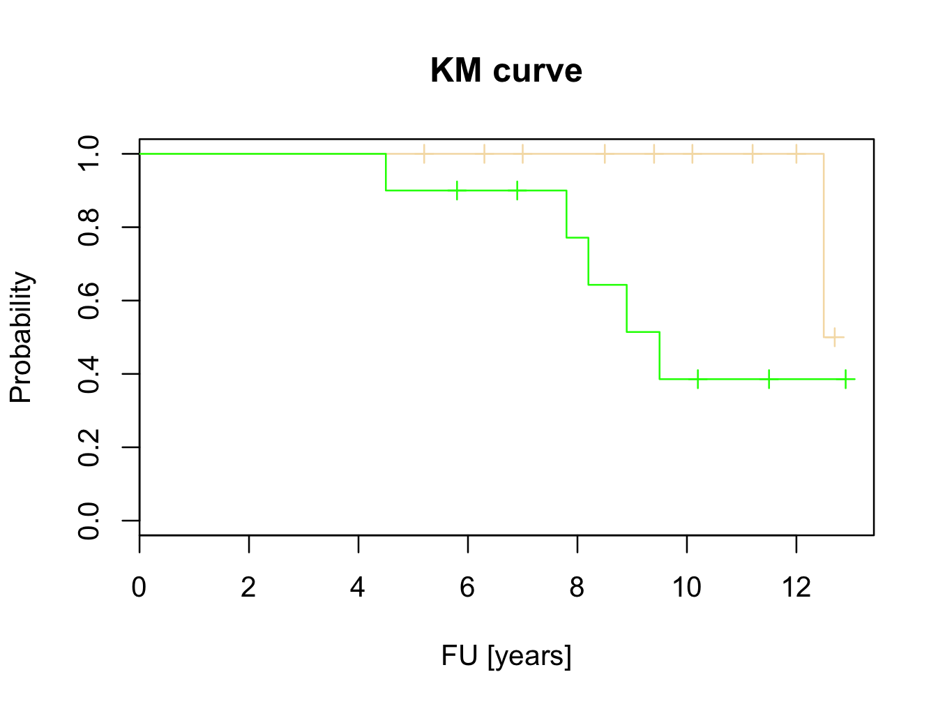 These results suggest that Hip 1 is superior to Hip 2. However, this will be tested with the logrank test, Cox proportional hazards and parametric tests.
Logrank test
The log rank test is a test that compares two survival curves. The null hypothesis is that the curves are identical. The statistical method uses a Chi Square test in its calculation. To perform this test in JGR / R is straight forward. The function that does the test is called “survdiff” (survival difference). Previously, the survival object was defined as mysurvival, but it is redefined (just in case) and its contents checked:
mysurvival<-Surv(plotsurvival$fu,plotsurvival$censor)
mysurvival
[1] 5.2+ 6.3+ 7.0+ 8.5+ 9.4+ 10.1+ 11.2+ 12.0+ 12.5 12.7+ 4.5 5.8+ 6.9+ 7.8 8.2 8.9 9.5 10.2+ 11.5+ 12.9+
To perform the log rank test:
mylogrank=survdiff(mysurvival~plotsurvival$group)
mylogrank
Call:
survdiff(formula = mysurvival ~ plotsurvival$group)
N Observed Expected (O-E)^2/E (O-E)^2/V
plotsurvival$group=Hip 1 10 1 3.31 1.61 3.63
plotsurvival$group=Hip 2 10 5 2.69 1.97 3.63
Chisq= 3.6 on 1 degrees of freedom, p= 0.0568
The p value is just larger than 5% and therefore the null hypothesis can’t be rejected. Although the curve suggests that Hip 2 performs worse than Hip 1, this can’t be confirmed statistically. However, there were only 10 patients in each group and the test lacks statistical power. Perhaps a more powerful test can show a difference (such as Cox proportional hazards or a parametric test; see below).
Cox proportional hazards
The cox proportional hazards test is a non parametric test that compares two or more survival curves. It is commonly used in medicine and more powerful than the log rank test. The function that performs this test in R is called “coxph”. The test is performed on the previously defined mysuvival object and the syntax is very similar to the log rank test:
mycoxproportionalhazards<-coxph(mysurvival~plotsurvival$group)
mycoxproportionalhazards
Call:
coxph(formula = mysurvival ~ plotsurvival$group)
coef exp(coef) se(coef) z p
plotsurvival$groupHip 2 1.84 6.28 1.10 1.67 0.095
Likelihood ratio test=3.84 on 1 df, p=0.05
n= 20, number of events= 6
The Cox proportional hazard test shows a statistical significant difference (just!). Therefore, the Cox proportional hazards test rejects the null hypothesis in favour of the alternate hypothesis and it is concluded that Hip 1 outperforms Hip 2. Please refer to the section on Cox proportional hazards for more information about this linear regression model.
Parametric
Parametric regression analysis can also be used to compare different survival curves. This method is more powerful than the methods describe above. However, it makes assumptions about the shape of the hazard function, which may or may not be justified. Assumptions of different types of hazard curves include (amongst others):
- Constant hazard (“exponential”), a constant hazard gives an exponential distribution.
- Increasing hazard, hazard increases as time goes on.
- Decreasing hazard, the hazard decreases as time goes on.
The R function ‘survreg’, that performs parametric regression analysis on survival curves, includes attributes for several distributions. These include: ‘weibull’, ‘exponential’, ‘gaussian’, ‘logistic’,’lognormal’ and ‘loglogistic’. A description is outside the scope of this book. Further information can be obtained from the build in help function. To perform regression analysis on the example is similar to the other tests and based on the mysurvival object:
Model 1: assume a constant hazard (exponential distribution):
myexponential<-survreg(mysurvival~plotsurvival$group,dist=’exponential’)
myexponential
Call:
survreg(formula = mysurvival ~ plotsurvival$group, dist = “exponential”)
Coefficients:
(Intercept) plotsurvival$groupHip 2
4.552824 -1.705591
Scale fixed at 1
Loglik(model)= -24.8 Loglik(intercept only)= -26.4
Chisq= 3.31 on 1 degrees of freedom, p= 0.069
n= 20
So, if a constant hazard is assumed, p>5% and the null hypothesis can’t be rejected. It must be concluded that there is no difference between the two hips. However, it is unlikely that the hazard remains constant over time. It is much more likely that the hazard for aseptic loosening increases over time. Therefore, it seems more appropriate to use a model such as Weibull:
Model 2: Weibull, increasing hazard over time:
myweibull<-survreg(mysurvival~plotsurvival$group,dist=’weibull’)
myweibull
Call:
survreg(formula = mysurvival ~ plotsurvival$group, dist = “weibull”)
Coefficients:
(Intercept) plotsurvival$groupHip 2
2.9364589 -0.5055782
Scale= 0.2617896
Loglik(model)= -20 Loglik(intercept only)= -22.2
Chisq= 4.31 on 1 degrees of freedom, p= 0.038
n= 20
The Weibull model clearly reaches statistical significance and the null hypothesis can be rejected in favour of the alternate hypothesis. It can be concluded that hip 1 is better than hip 2.
Cox proportional hazards or parametric regression analysis?
Both, parametric and non parametric analysis may be appropriate to use to demonstrate a difference between two groups. Parametric regression analysis is more powerful, but makes assumptions regarding the shape of the hazard function. This may not always be appropriate. Parametric regression analysis defines the shape of the hazard function and therefore allows for extrapolation. This is not possible with the Cox proportional hazards model.
Traditionally, medical studies tend to use the Cox proportional hazards model whilst engineering uses the parametric regression analysis. However, parametric analysis can easily be applied to medicine and this can be particularly useful if prediction / extrapolation is required.
Hazard plot
This function requires the muhaz 3 package to be installed and loaded. The hazard function is related to the survival function and can be derived from it. Given the patient has survived up to a certain time, the hazard function gives the instantaneous hazard for the event to happen at that time. Hazard plots can be very useful in estimating the risk of the event of interest occurring, given the patient has survived up to that time. Still using the same example, the muhaz function does this conveniently. Enter the following in the JGR R command window:
library(muhaz)
myhazard<-muhaz(plotsurvival$fu,plotsurvival$censor,max.time=4)
plot(myhazard)
title(main=’Hazard Plot’)
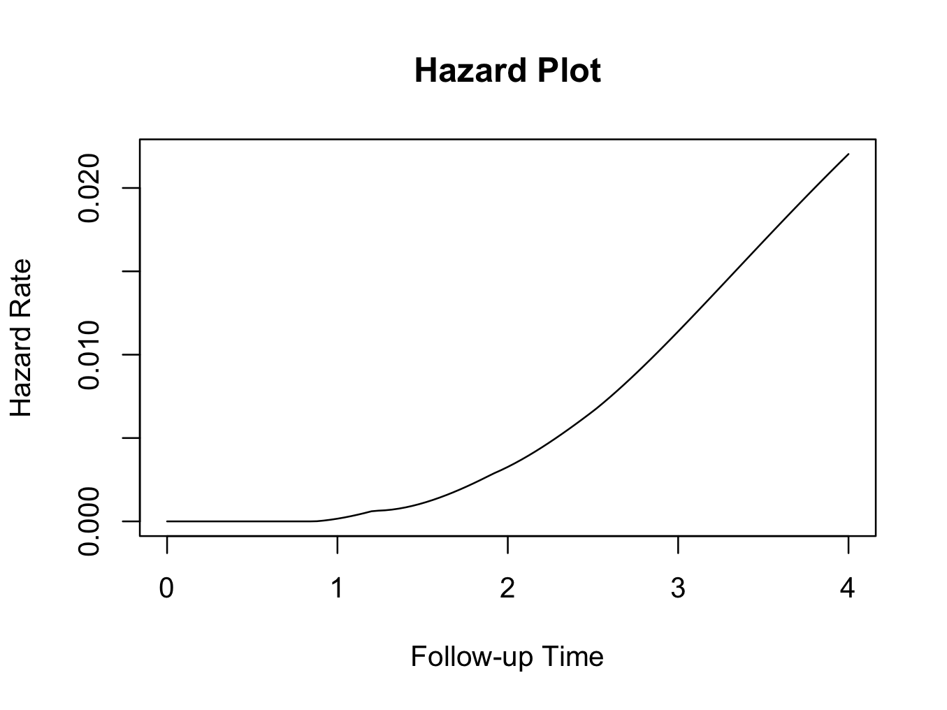
The plot clearly shows that the hazard of failure increases over time, suggesting that it would be appropriate to use the parametric Weibull analysis as described above.
Kaplan-Meier plot showing numbers at risk
It may be preferable to have the number of patients at risk indicated in the plot. The KMatRisk function can be used for this. Copy the function to the clipboard, paste it into the console and hit return. The function should now be available in R (the library survival 1 should also be installed and loaded).
Create the survival curve object directly (in one step) from the data and call this hipfit:
hipfit<-survfit(Surv(fu,censor)~group,data=plotsurvival)
Next call the loaded function to create the survival curve with numbers at risk:
ggkm(hipfit,timeby=1,ystratalabs=c(“Hip 1″,”Hip 2″),main=”KM plot, Hip by type”,xlabs=”FU [Years]”)
The above code can be copied and pasted into the console, but the special characters (” or ‘) may need to be re-entered.
Prodlim package
The prodlim 4 package should be installed. The package creates nice survival curves. First install the library:
library(prodlim)
Create a Kaplan-Meier object using the product limit method:
kmhipfit <- prodlim(Hist(fu, censor) ~ 1, data = plotsurvival)
To create a plot that shows numbers at risk at yearly intervals with a shadowed 95% confidence interval:
plot(kmhipfit,percent=FALSE,axes=TRUE,axis1.at=seq(0,kmhipfit$maxtime+1,1),axis1.lab=seq(0,kmhipfit$maxtime+1,1),marktime=TRUE,xlab=”Years”,atrisk=TRUE,atrisk.labels=”At Risk:”,confint=TRUE,confint.citype=”shadow”,col=4)
And add a title:
title(main= “Kaplan Meier Survival Analysis – All Hips”)
 Similarly, create a plot grouped by type of hip replacement (instead of ~1, use ~group):
kmhipfit2 <- prodlim(Hist(fu, censor) ~ group, data = plotsurvival)
plot(kmhipfit2,percent=FALSE,axes=TRUE,axis1.at=seq(0,kmhipfit2$maxtime+1,1),axis1.lab=seq(0,kmhipfit2$maxtime+1,1),marktime=TRUE,xlab=”Years”,atrisk=TRUE,atrisk.labels=”At Risk:”,confint=TRUE,confint.citype=”shadow”,col=c(4,3),legend=TRUE,legend.x=0,legend.y=0.4,legend.cex=1)
title(main= “Kaplan Meier Survival Analysis – By Hip Type”)
 For more information re prodlim options:
??prodlim
Please note the syntax to place the legend position.
Other packages that can be of use in creating survival curves are the survminer 5 and the ggfortify 6 packages (autoplot() function) that are designed to work with ggplot2 7.