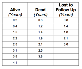
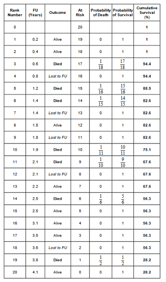
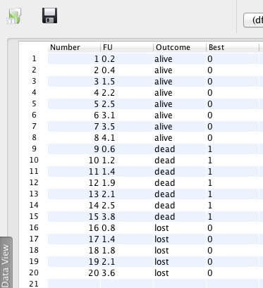
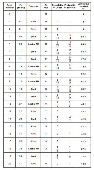
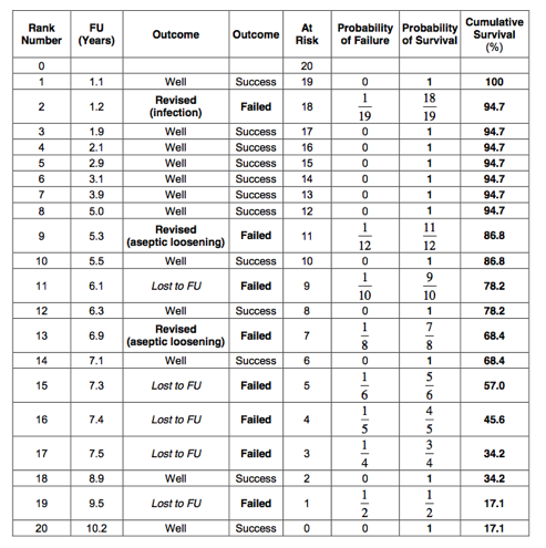
The table below shows 20 patients who have been diagnosed with cancer. The first column shows the follow up (in years) of the patients who were alive at review. In the second column, the follow up till time of death is indicated. The third column shows the time to last review in the patients who were lost to follow up:
The data is also available in Q9.rda and for convenience the table is shown below:
- Calculate the 5-year survival in the best-case scenario, using life table analysis.
The best-case scenario is as follows:
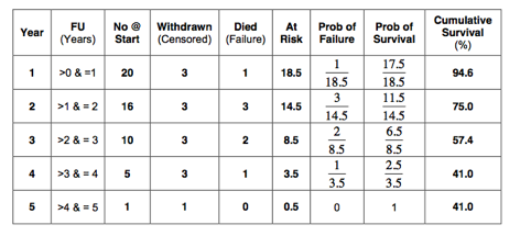 So, the 5-year survival in the best-case scenario as estimated with life table analysis is 41%.
- Calculate the 5-year survival in the worst-case scenario, using life table analysis.
The worst-case scenario life table is as follows:
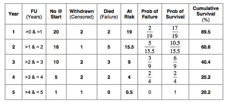 So, the 5-year survival in the worst-case scenario as estimated with life table analysis is 20%.
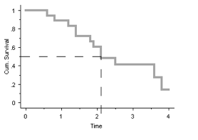
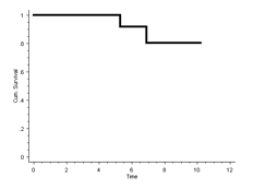
- Show the best-case scenario and worst-case scenario survival curves in 1 graph, using life table analysis.
Using the tables constructed in Q1 and Q2, survival curves can be drawn:
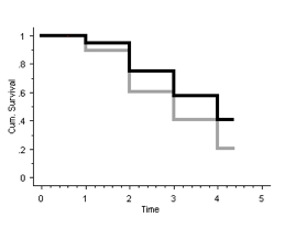 The best-case scenario is shown in black and the worst-case scenario is shown in grey.
- Perform the Kaplan-Meier survival analysis in the best-case scenario.
In the best-case scenario, the patients lost to follow up count as a success. The Kaplan-Meier table is as follows:
In R / JGR:
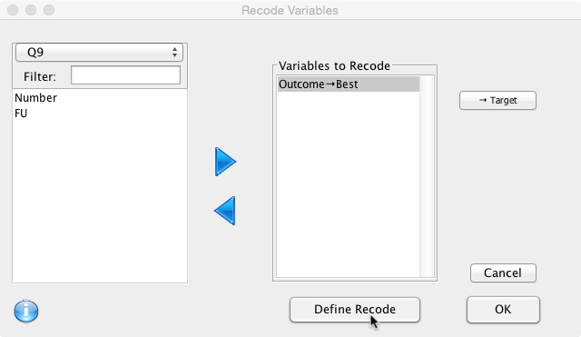
Once the data frame is loaded, the data should be visible in the Data Viewer with the variables ‘Number’, ‘FU’ and ‘Outcome’. It is of course possible to create a new logical variable (called ‘Best’) and go through the data manually, setting the value to FALSE if the ‘Outcome’ variable is ‘alive’ or ‘lost’ and TRUE if the ‘Outcome’ variable is ‘dead’. However, this would become tedious for larger data sets. For larger data sets it would be easier to recode the variable ‘Outcome’ in a new variable (called ‘Best’). Select ‘Data’ and then ‘Recode Variables’ from the menu bar. In the dialogue box, select the variable ‘Outcome’ to recode and define the Target as ‘Best':

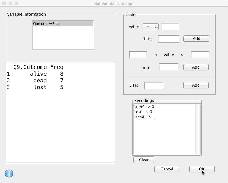
Next define the recode as 0 when the ‘Outcome’ variable is ‘alive’ or ‘lost’ and 1 when it is ‘dead':
Click OK
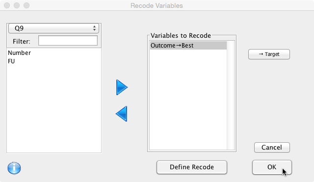
And click OK again
This should show the recoded new variable ‘Best’ in the Data Viewer:
However, because the ‘Outcome’ variable is a ‘Factor’ (categorical data), the new variable ‘Best’ is also defined as a ‘Factor’ rather than ‘Logical’ or ‘Integer’ that is required for survival analysis! Therefore, it is necessary to convert the variable ‘Best’ from a ‘Factor’ to an ‘Integer’. This can be done by clicking on the ‘Variable View’ tab in the Data Viewer. However, this converts the zeros to a 1 and a 1 to a 2 (the factor levels)! Although it is possible to perform survival analysis with the outcome variable as 1 and 2 rather than 0 and 1, it is somewhat illogical. Therefore, recode the ‘Best’ variable again into itself, setting 1 to 0 and 2 to 1.

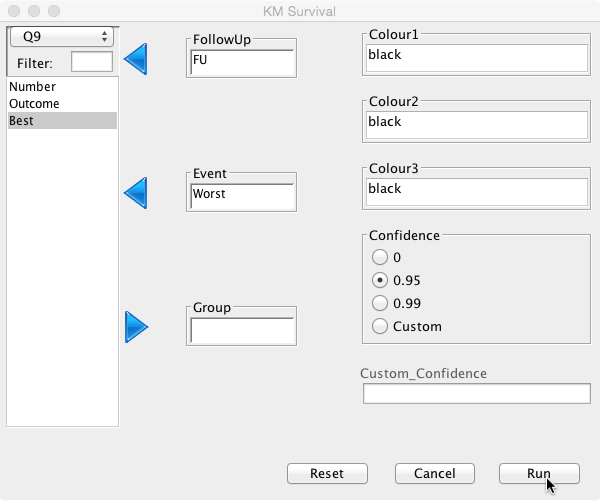
Now perform the survival analysis using DeducerSurvival 1. Make sure the package DeducerSurvival is installed. From the Deducer menu bar, select ‘Survival’ and then ‘Kaplan Meier’. In the dialogue box, select ‘FU’ as ‘FollowUp’ and ‘Best’ as ‘Event':
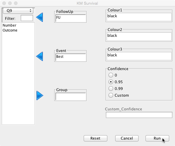
Click Run should give the following console output and plot:
mySurvival = with( Q9 , Surv( FU , Best ))
summary(mySurvival)
time status
Min. :0.200 Min. :0.00
1st Qu.:1.350 1st Qu.:0.00
Median :2.000 Median :0.00
Mean :2.035 Mean :0.35
3rd Qu.:2.650 3rd Qu.:1.00
Max. :4.100 Max. :1.00
mycurve=survfit(mySurvival~1,conf.int= 0.95 )
summary(mycurve)
Call: survfit(formula = mySurvival ~ 1, conf.int = 0.95)
time n.risk n.event survival std.err lower 95% CI upper 95% CI
0.6 18 1 0.944 0.0540 0.8443 1.000
1.2 16 1 0.885 0.0763 0.7477 1.000
1.4 15 1 0.826 0.0913 0.6655 1.000
1.9 11 1 0.751 0.1096 0.5644 1.000
2.1 10 1 0.676 0.1217 0.4751 0.962
2.5 7 1 0.580 0.1374 0.3642 0.922
3.8 2 1 0.290 0.2161 0.0672 1.000
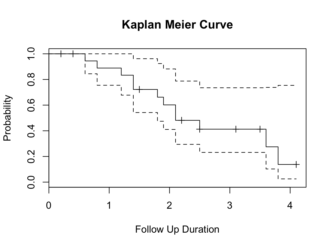
plot(mycurve, col=c( ” black ” , ” black ” , ” black ” ))
title(main= “Kaplan Meier Curve” ,xlab= “Follow Up Duration” ,ylab= “Probability” )
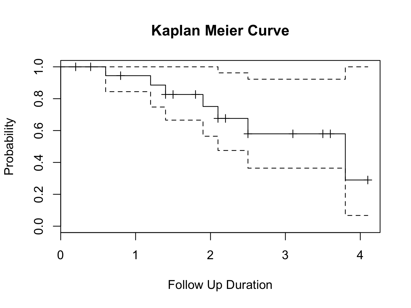
Please note the survival estimate is similar to the table above, but the last two values are slightly different due to rounding error.
- What is the survival in Q4 at 4.1 years?
The survival at 4.1 years in the best-case scenario as estimated with Kaplan-Meier analysis is 28%.
In R / JGR:
Using the table in Q4: 29%.
Or alternatively in the console on the recoded variable ‘Best':
mysurvival<-Surv(Q9$FU,Q9$Best)
mysurvival
[1] 0.2+ 0.4+ 1.5+ 2.2+ 2.5+ 3.1+ 3.5+ 4.1+ 0.6 1.2 1.4 1.9 2.1 2.5 3.8 0.8+ 1.4+ 1.8+ 2.1+ 3.6+
mycurve<-survfit(mysurvival~1)
mycurve
Call: survfit(formula = mysurvival ~ 1)
n events median 0.95LCL 0.95UCL
20.0 7.0 3.8 2.1 NA
summary(mycurve,time=4.1)
Call: survfit(formula = mysurvival ~ 1)
time n.risk n.event survival std.err lower 95% CI upper 95% CI
4.1 1 7 0.29 0.216 0.0672 1
Therefore, the survival at 4.1 years is 29%.
- What is the median survival in Q4?
For the answer to this question we need to plot the survival curve:
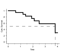 It can be seen from the graph that the median survival ≈ 3.75 years.
In R / JGR:
The median survival is not provided when using DeducerSurvival. It can be estimated from the plot as described above. Alternatively, using the console method (as above):
mysurvival<-Surv(Q9$FU,Q9$Best)
mysurvival
[1] 0.2+ 0.4+ 1.5+ 2.2+ 2.5+ 3.1+ 3.5+ 4.1+ 0.6 1.2 1.4 1.9 2.1 2.5 3.8 0.8+ 1.4+ 1.8+ 2.1+ 3.6+
mycurve<-survfit(mysurvival~1)
mycurve
Call: survfit(formula = mysurvival ~ 1)
n events median 0.95LCL 0.95UCL
20.0 7.0 3.8 2.1 NA
Therefore, the median survival is 3.8 years.
- Perform the Kaplan-Meier survival analysis in the worst-case scenario.
In the worst-case scenario, the patients lost to follow up count as a failure. The Kaplan-Meier table is as follows:
In R / JGR:
Similarly as in Q4, the ‘Outcome’ variable can be recoded into a new variable ‘Worst'; when the ‘Outcome’ is ‘alive’ ‘Worst’ is coded as 0 and when the ‘Outcome’ is ‘dead’ or ‘lost’ ‘Worst’ is coded as 1:

Again, convert the variable type from Factor to Integer and recode again as described above to convert 2 to 1 and 1 to zero:

Next perform the survival analysis with DeducerSurvival as described above.
This should give the following output and plot:
mySurvival = with( Q9 , Surv( FU , Worst ))
summary(mySurvival)
time status
Min. :0.200 Min. :0.0
1st Qu.:1.350 1st Qu.:0.0
Median :2.000 Median :1.0
Mean :2.035 Mean :0.6
3rd Qu.:2.650 3rd Qu.:1.0
Max. :4.100 Max. :1.0
mycurve=survfit(mySurvival~1,conf.int= 0.95 )
summary(mycurve)
Call: survfit(formula = mySurvival ~ 1, conf.int = 0.95)
time n.risk n.event survival std.err lower 95% CI upper 95% CI
0.6 18 1 0.944 0.0540 0.8443 1.000
0.8 17 1 0.889 0.0741 0.7549 1.000
1.2 16 1 0.833 0.0878 0.6778 1.000
1.4 15 2 0.722 0.1056 0.5423 0.962
1.8 12 1 0.662 0.1126 0.4743 0.924
1.9 11 1 0.602 0.1174 0.4107 0.882
2.1 10 2 0.481 0.1209 0.2944 0.788
2.5 7 1 0.413 0.1216 0.2316 0.735
3.6 3 1 0.275 0.1385 0.1026 0.738
3.8 2 1 0.138 0.1194 0.0251 0.754
plot(mycurve, col=c( ” black ” , ” black ” , ” black ” ))
title(main= “Kaplan Meier Curve” ,xlab= “Follow Up Duration” ,ylab= “Probability” )
- What is the survival in Q7 at 4.1 years?
The survival at 4.1 years in the worst-case scenario as estimated with Kaplan-Meier analysis is 14%.
In R / JGR:
Using the table in Q7: 13.8%.
Or alternatively in the console on the recoded variable ‘Worst':
mysurvival<-Surv(Q9$FU,Q9$Worst)
mysurvival
[1] 0.2+ 0.4+ 1.5+ 2.2+ 2.5+ 3.1+ 3.5+ 4.1+ 0.6 1.2 1.4 1.9 2.1 2.5 3.8 0.8 1.4 1.8 2.1 3.6
mycurve<-survfit(mysurvival~1)
mycurve
Call: survfit(formula = mysurvival ~ 1)
n events median 0.95LCL 0.95UCL
20.0 12.0 2.1 1.8 NA
summary(mycurve,time=4.1)
Call: survfit(formula = mysurvival ~ 1)
time n.risk n.event survival std.err lower 95% CI upper 95% CI
4.1 1 12 0.138 0.119 0.0251 0.754
Therefore, the survival at 4.1 years is 13.8%.
- What is the median survival in Q7?
For the answer to this question we need to plot the survival curve:
 It can be estimated from the graph that the median survival ≈ 2.25 years.
Or in R / JGR:
mysurvival<-Surv(Q9$FU,Q9$Worst)
mysurvival
[1] 0.2+ 0.4+ 1.5+ 2.2+ 2.5+ 3.1+ 3.5+ 4.1+ 0.6 1.2 1.4 1.9 2.1 2.5 3.8 0.8 1.4 1.8 2.1 3.6
mycurve<-survfit(mysurvival~1)
mycurve
Call: survfit(formula = mysurvival ~ 1)
n events median 0.95LCL 0.95UCL
20.0 12.0 2.1 1.8 NA
Therefore, the median survival is 2.1 years.
The outcome data of 20 patients who had a total ankle replacement are listed in survivalankle.rda.
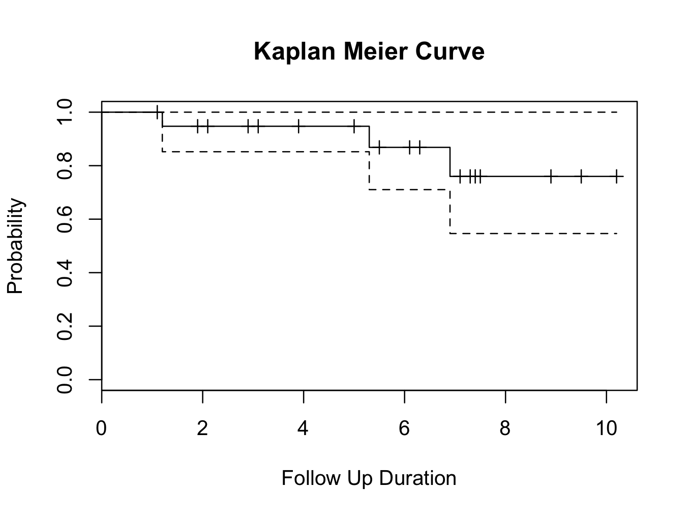
- Calculate the 10-year Kaplan-Meier survival of the prosthesis using revision for aseptic loosening as ‘hard end point’.
Only patients who had a ‘Revision’ for aseptic loosening are counted as failures. The Kaplan-Meier table is as follows:
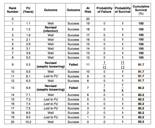 The 10-year Kaplan-Meier survival for aseptic loosening is therefore 80%:
Or in JGR / R:
First recode the ‘Outcome’ variable to a variable called ‘Censor’ as described above (Q4).

Then, as before, convert the Censor variable to ‘Integer’ and recode again to convert the 1 to 0 and 2 to 1.

Finally, perform the analysis with DeducerSurvival should result in the following output:
mySurvival = with( survivalankle , Surv( FU , Censor ))
summary(mySurvival)
time status
Min. : 1.100 Min. :0.0
1st Qu.: 3.050 1st Qu.:0.0
Median : 5.800 Median :0.0
Mean : 5.460 Mean :0.1
3rd Qu.: 7.325 3rd Qu.:0.0
Max. :10.200 Max. :1.0
mycurve=survfit(mySurvival~1,conf.int= 0.95 )
summary(mycurve)
Call: survfit(formula = mySurvival ~ 1, conf.int = 0.95)
time n.risk n.event survival std.err lower 95% CI upper 95% CI
5.3 12 1 0.917 0.0798 0.773 1
6.9 8 1 0.802 0.1279 0.587 1
plot(mycurve, col=c( ” black ” , ” black ” , ” black ” ))
title(main= “Kaplan Meier Curve” ,xlab= “Follow Up Duration” ,ylab= “Probability” )
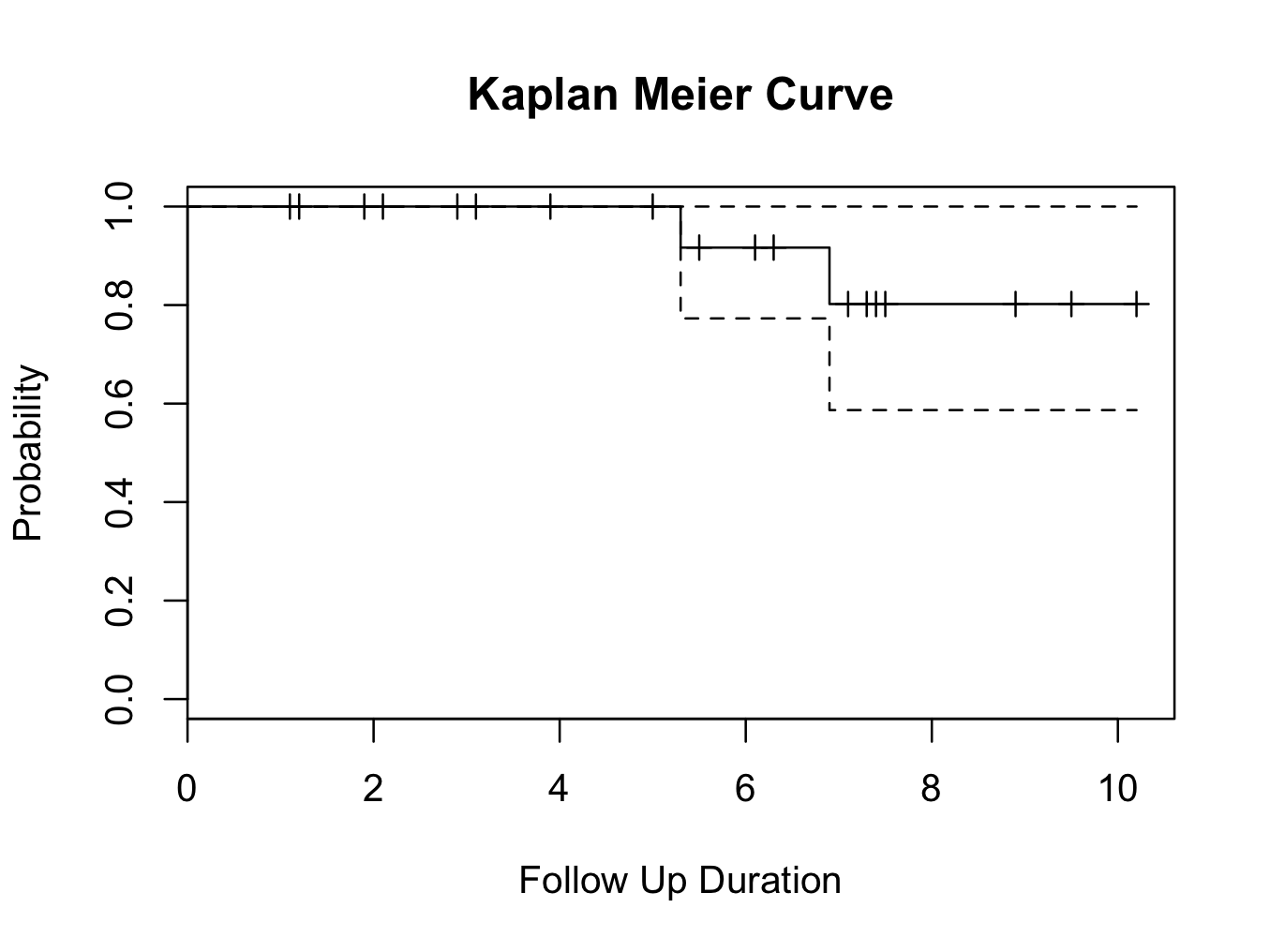 Therefore, the 10 year survival is 80%.
In the console:
mysurvival<-Surv(survivalankle$FU,survivalankle$Censor)
mysurvival
[1] 1.1+ 1.2+ 1.9+ 2.1+ 2.9+ 3.1+ 3.9+ 5.0+ 5.3 5.5+ 6.1+ 6.3+ 6.9 7.1+ 7.3+ 7.4+ 7.5+ 8.9+ 9.5+ 10.2+
mycurve<-survfit(mysurvival~1)
mycurve
Call: survfit(formula = mysurvival ~ 1)
n events median 0.95LCL 0.95UCL
20 2 NA NA NA
summary(mycurve,time=10)
Call: survfit(formula = mysurvival ~ 1)
time n.risk n.event survival std.err lower 95% CI upper 95% CI
10 1 2 0.802 0.128 0.587 1
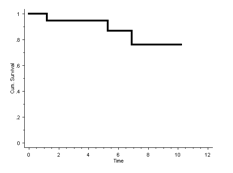
- Calculate the 10-year Kaplan-Meier survival of the prosthesis using revision as ‘hard end point’.
All patients who had a ‘Revision’ are counted as failures. The Kaplan-Meier table is as follows:
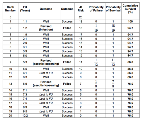 The 10-year Kaplan-Meier survival for revision is therefore 76%:
Or in JGR / R:
Perform recoding similar as to above into a new variable ‘Censor2′, but now counting all revisions as failures and perform the analysis in DeducerSurvival:
mySurvival = with( survivalankle , Surv( FU , Censor2 ))
summary(mySurvival)
time status
Min. : 1.100 Min. :0.00
1st Qu.: 3.050 1st Qu.:0.00
Median : 5.800 Median :0.00
Mean : 5.460 Mean :0.15
3rd Qu.: 7.325 3rd Qu.:0.00
Max. :10.200 Max. :1.00
mycurve=survfit(mySurvival~1,conf.int= 0.95 )
summary(mycurve)
Call: survfit(formula = mySurvival ~ 1, conf.int = 0.95)
time n.risk n.event survival std.err lower 95% CI upper 95% CI
1.2 19 1 0.947 0.0512 0.852 1
5.3 12 1 0.868 0.0890 0.710 1
6.9 8 1 0.760 0.1280 0.546 1
plot(mycurve, col=c( ” black ” , ” black ” , ” black ” ))
title(main= “Kaplan Meier Curve” ,xlab= “Follow Up Duration” ,ylab= “Probability” )
 Therefore, the 10 year survival is 76%.
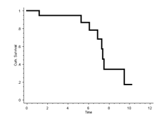
- Calculate the 10-year worst-case scenario Kaplan-Meier survival of the prosthesis using revision as ‘hard end point’.
In the worst-case scenario, all patients who are lost to follow up are also counted as a failure:
 The worst-case scenario 10-year Kaplan-Meier survival for revision is therefore 17%:
Or in JGR / R:
Again, perform recoding similar to above into a new variable called ‘Censor3′, now counting all revisions and all patients lost to follow up as a failure.

As above, change to an integer variable and recode again to convert 1 to 0 and 2 to 1. Using DeducerSurvial, the result is:
mySurvival = with( survivalankle , Surv( FU , Censor3 ))
summary(mySurvival)
time status
Min. : 1.100 Min. :0.0
1st Qu.: 3.050 1st Qu.:0.0
Median : 5.800 Median :0.0
Mean : 5.460 Mean :0.4
3rd Qu.: 7.325 3rd Qu.:1.0
Max. :10.200 Max. :1.0
mycurve=survfit(mySurvival~1,conf.int= 0.95 )
summary(mycurve)
Call: survfit(formula = mySurvival ~ 1, conf.int = 0.95)
time n.risk n.event survival std.err lower 95% CI upper 95% CI
1.2 19 1 0.947 0.0512 0.8521 1.000
5.3 12 1 0.868 0.0890 0.7104 1.000
6.1 10 1 0.782 0.1149 0.5859 1.000
6.9 8 1 0.684 0.1359 0.4633 1.000
7.3 6 1 0.570 0.1538 0.3358 0.967
7.4 5 1 0.456 0.1598 0.2294 0.906
7.5 4 1 0.342 0.1552 0.1404 0.833
9.5 2 1 0.171 0.1437 0.0329 0.888
plot(mycurve, col=c( ” black ” , ” black ” , ” black ” ))
title(main= “Kaplan Meier Curve” ,xlab= “Follow Up Duration” ,ylab= “Probability” )
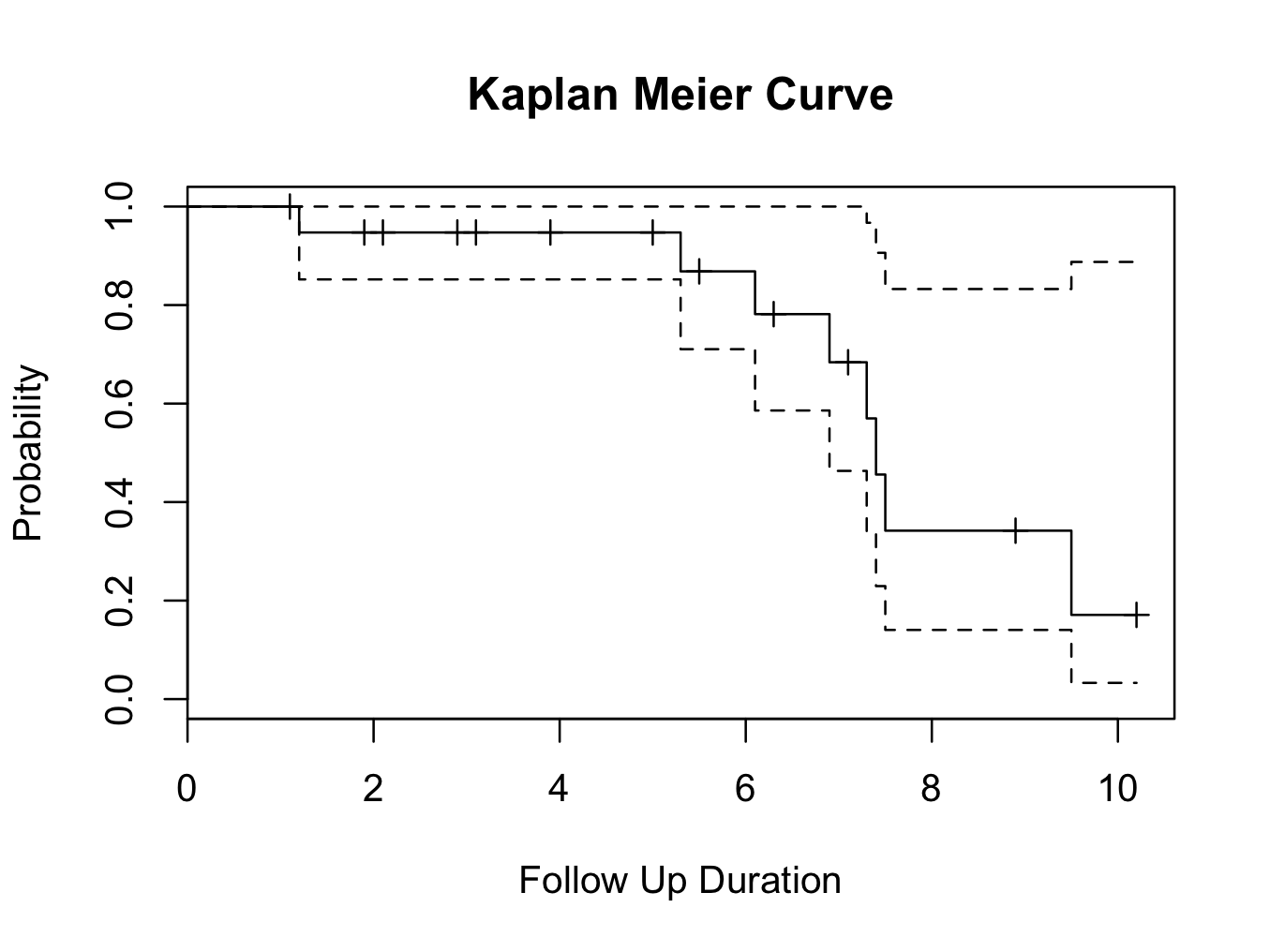 Again, giving the result 17%.
These questions illustrate the importance of choosing a ‘hard end point’. They also show that if all patients lost to follow up are counted as a failure (worst-case scenario), the survival curve drops steeply.
There was not much difference in the 10-year survival for ‘revision’ and ‘revision for aseptic loosening’. This is because the one patient who had an infection had this relatively early (at 1.2 years). At this time there were 18 patients who had a longer follow up. Consequently, the effect on the failure rate (1 out of 19) is not as big as it would have been if only 1 patient had a longer follow up (1 out of 2).
So, a failure at the ‘tail end’ (longer follow up) of the survival curve has a far more pronounced effect on the cumulative survival than a failure at the beginning (short follow up).
In the DeducerSurvival interface: Select the survivalhip1 data frame, with FU as FollowUp variable, Censor as Event and Group as Group. In the ‘Colour1′ box enter ‘brown’ and in the ‘Colour2′ box ‘blue’. The ‘Colour3′ box can be left as its default value (black). There is no need to change the confidence interval as these are not included in grouped survival curves. Hit ‘Run':
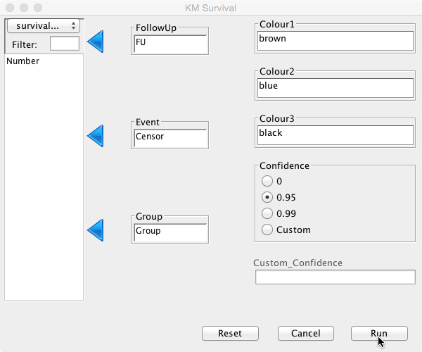
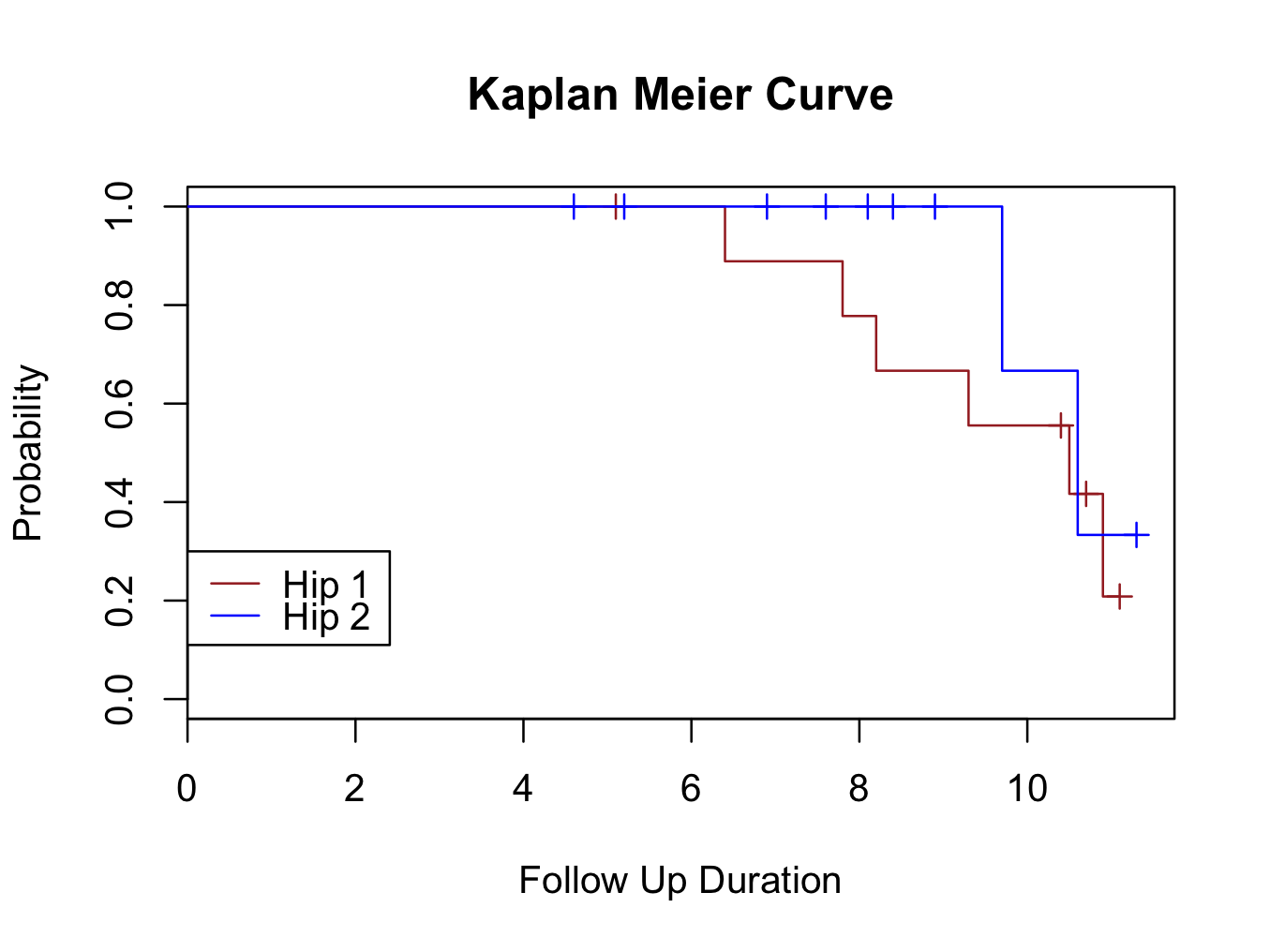
This should generate the survival curve:
 The following output is generated in the console:
mySurvival = with( survivalhip1 , Surv( FU , Censor ))
summary(mySurvival)
time status
Min. : 4.600 Min. :0.0
1st Qu.: 7.425 1st Qu.:0.0
Median : 8.650 Median :0.0
Mean : 8.585 Mean :0.4
3rd Qu.:10.525 3rd Qu.:1.0
Max. :11.300 Max. :1.0
mycurve=with( survivalhip1 , survfit(mySurvival~ Group ,conf.int= 0.95 ))
summary(mycurve)
Call: survfit(formula = mySurvival ~ Group, conf.int = 0.95)
Group=Hip 1
time n.risk n.event survival std.err lower 95% CI upper 95% CI
6.4 9 1 0.889 0.105 0.7056 1.000
7.8 8 1 0.778 0.139 0.5485 1.000
8.2 7 1 0.667 0.157 0.4200 1.000
9.3 6 1 0.556 0.166 0.3097 0.997
10.5 4 1 0.417 0.173 0.1847 0.940
10.9 2 1 0.208 0.171 0.0418 1.000
Group=Hip 2
time n.risk n.event survival std.err lower 95% CI upper 95% CI
9.7 3 1 0.667 0.272 0.2995 1
10.6 2 1 0.333 0.272 0.0673 1
Sometimes, DeducerSurvival labels the curves incorrectly and it is necessary to check the curves are correct. From the output above, it can be seen that there were 6 failures in ‘Hip 1′ and two failures in ‘Hip 2′. Therefore, There should be 6 steps in the brown curve and only two in the blue which is correct. The drops in the curve are steeper for ‘Hip 2′ because 7 patients were censored at the time of the first failure.
Using the console:
library(survival)
mysurvival<-Surv(survivalhip1$FU,survivalhip1$Censor)
mysurvival
[1] 5.1+ 6.4 7.8 8.2 9.3 10.4+ 10.5 10.7+ 10.9 11.1+ 4.6+ 5.2+ 6.9+ 7.6+ 8.1+ 8.4+ 8.9+ 9.7 10.6 11.3+
mycurve<-survfit(mysurvival~survivalhip1$Group)
mycurve
Call: survfit(formula = mysurvival ~ survivalhip1$Group)
n events median 0.95LCL 0.95UCL
survivalhip1$Group=Hip 1 10 6 10.5 8.2 NA
survivalhip1$Group=Hip 2 10 2 10.6 9.7 NA
summary(mycurve)
Call: survfit(formula = mysurvival ~ survivalhip1$Group)
survivalhip1$Group=Hip 1
time n.risk n.event survival std.err lower 95% CI upper 95% CI
6.4 9 1 0.889 0.105 0.7056 1.000
7.8 8 1 0.778 0.139 0.5485 1.000
8.2 7 1 0.667 0.157 0.4200 1.000
9.3 6 1 0.556 0.166 0.3097 0.997
10.5 4 1 0.417 0.173 0.1847 0.940
10.9 2 1 0.208 0.171 0.0418 1.000
survivalhip1$Group=Hip 2
time n.risk n.event survival std.err lower 95% CI upper 95% CI
9.7 3 1 0.667 0.272 0.2995 1
10.6 2 1 0.333 0.272 0.0673 1
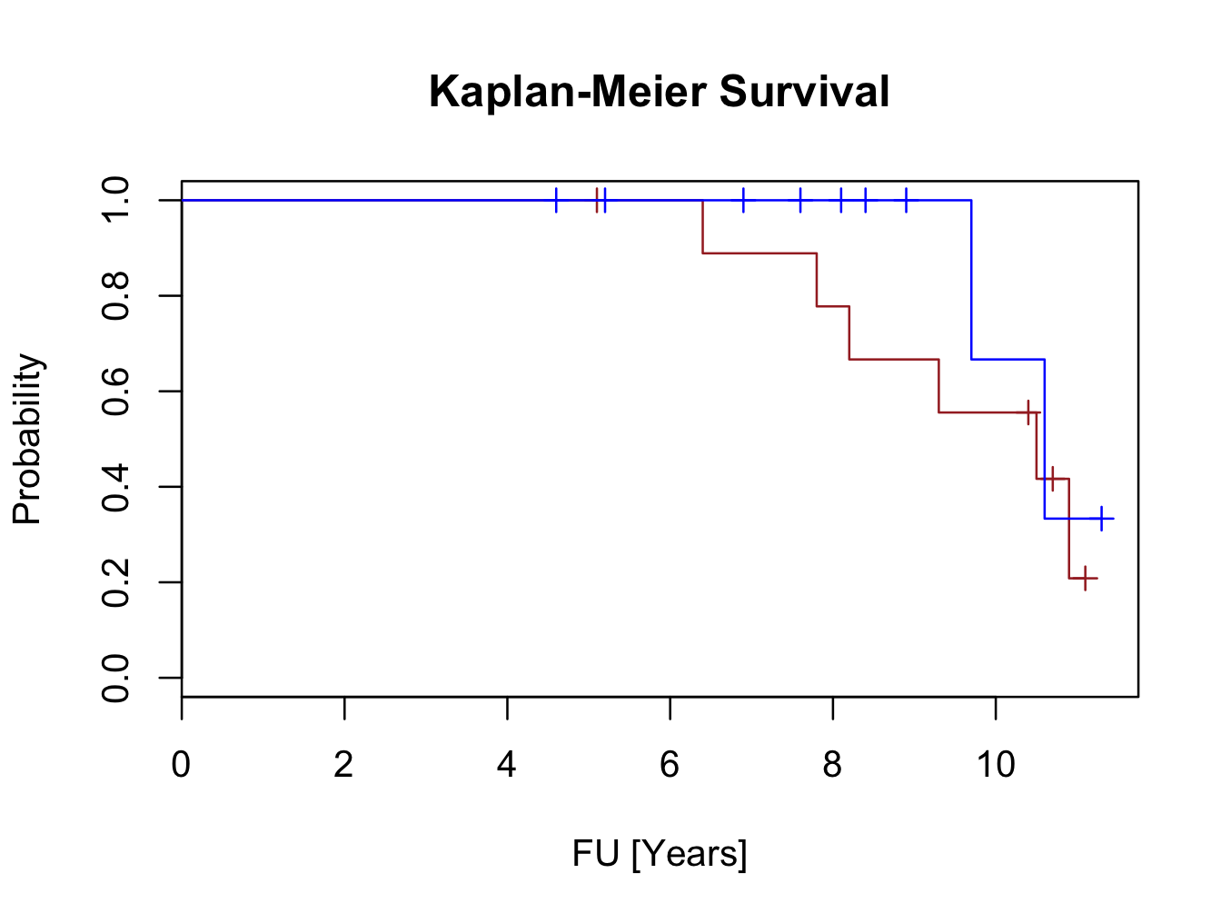
plot(mycurve,col=c(“brown”,”blue”))
title(main=”Kaplan-Meier Survival”,xlab=”FU [Years]”,ylab=”Probability”)
In the DeducerSurvival interface:
After the survival curves have been plotted (Q13), select ‘Survival’ followed by ‘Compare’ from the Deducer GUI. In the dialogue box, select the survivalhip1 data frame, with FU as FollowUp variable, Censor as Event and Group as Group. Make sure ‘Weibull’ is selected under ‘Parametric’ (you can’t select two parametric tests and the exponential test will have to be done sequentially) and ‘Run’ under ‘NonParametric’.
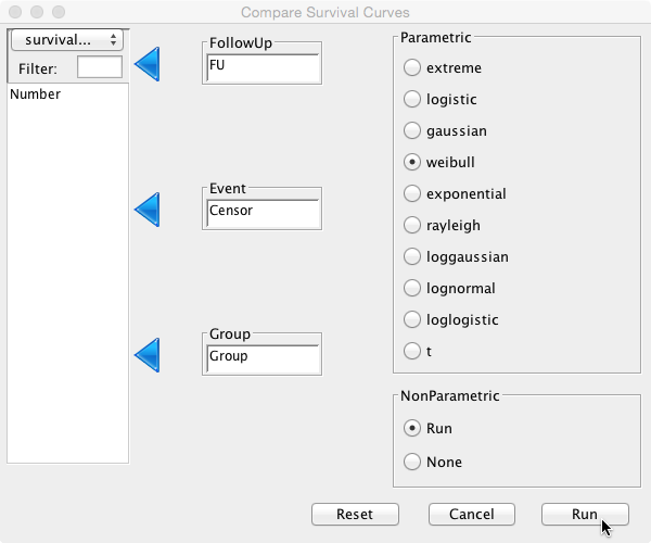
Click ‘Run’ and the following output should be generated in the console:
mySurvival = with( survivalhip1 , Surv( FU , Censor ))
mylogrank=with( survivalhip1 , survdiff(mySurvival~ Group ))
mylogrank
Call:
survdiff(formula = mySurvival ~ Group)
N Observed Expected (O-E)^2/E (O-E)^2/V
Group=Hip 1 10 6 4.91 0.242 0.634
Group=Hip 2 10 2 3.09 0.385 0.634
Chisq= 0.6 on 1 degrees of freedom, p= 0.426
mycoxph=with( survivalhip1 , coxph(mySurvival~ Group ))
mycoxph
Call:
coxph(formula = mySurvival ~ Group)
coef exp(coef) se(coef) z p
GroupHip 2 -0.642 0.526 0.820 -0.78 0.43
Likelihood ratio test=0.67 on 1 df, p=0.412
n= 20, number of events= 8
myparametric=with( survivalhip1 , survreg(mySurvival~ Group , dist = “weibull” ))
myparametric
Call:
survreg(formula = mySurvival ~ Group, dist = “weibull”)
Coefficients:
(Intercept) GroupHip 2
2.36525220 0.08988363
Scale= 0.1416005
Loglik(model)= -20.5 Loglik(intercept only)= -20.8
Chisq= 0.66 on 1 degrees of freedom, p= 0.42
n= 20
Similarly, perform the exponential parametric test which should show the following output (parts omitted for brevity):
myparametric=with( survivalhip1 , survreg(mySurvival~ Group , dist = “exponential” ))
myparametric
Call:
survreg(formula = mySurvival ~ Group, dist = “exponential”)
Coefficients:
(Intercept) GroupHip 2
2.712485 0.992514
Scale fixed at 1
Loglik(model)= -31.7 Loglik(intercept only)= -32.5
Chisq= 1.69 on 1 degrees of freedom, p= 0.19
n= 20
There is no statistical significant difference using the log rank test (p=0.426), cox proportional hazards model (p=0.412) and parametric regression analysis using the exponential (p=0.19) and Weibull (p=0.42) distributions between the survival curves of both hips. Therefore, the null hypothesis can’t be rejected and it should be concluded that there is no difference in the outcome of both hips.
Using the console:
Create the survival object again (already done in Q13) and perform the tests:
library(survival)
mysurvival<-Surv(survivalhip1$FU,survivalhip1$Censor)
mysurvival
[1] 5.1+ 6.4 7.8 8.2 9.3 10.4+ 10.5 10.7+ 10.9 11.1+ 4.6+ 5.2+ 6.9+ 7.6+ 8.1+ 8.4+ 8.9+ 9.7 10.6 11.3+
mylogrank<-survdiff(mysurvival~survivalhip1$Group)
mylogrank
Call:
survdiff(formula = mysurvival ~ survivalhip1$Group)
N Observed Expected (O-E)^2/E (O-E)^2/V
survivalhip1$Group=Hip 1 10 6 4.91 0.242 0.634
survivalhip1$Group=Hip 2 10 2 3.09 0.385 0.634
Chisq= 0.6 on 1 degrees of freedom, p= 0.426
mycox<-coxph(mysurvival~survivalhip1$Group)
mycox
Call:
coxph(formula = mysurvival ~ survivalhip1$Group)
coef exp(coef) se(coef) z p
survivalhip1$GroupHip 2 -0.642 0.526 0.820 -0.78 0.43
Likelihood ratio test=0.67 on 1 df, p=0.412
n= 20, number of events= 8
myexponential<-survreg(mysurvival~survivalhip1$Group,dist=”exponential”)
myexponential
Call:
survreg(formula = mysurvival ~ survivalhip1$Group, dist = “exponential”)
Coefficients:
(Intercept) survivalhip1$GroupHip 2
2.712485 0.992514
Scale fixed at 1
Loglik(model)= -31.7 Loglik(intercept only)= -32.5
Chisq= 1.69 on 1 degrees of freedom, p= 0.19
n= 20
myweibull<-survreg(mysurvival~survivalhip1$Group,dist=”weibull”)
myweibull
Call:
survreg(formula = mysurvival ~ survivalhip1$Group, dist = “weibull”)
Coefficients:
(Intercept) survivalhip1$GroupHip 2
2.36525220 0.08988363
Scale= 0.1416005
Loglik(model)= -20.5 Loglik(intercept only)= -20.8
Chisq= 0.66 on 1 degrees of freedom, p= 0.42
n= 20
There is no statistical significant difference using the log rank test (p=0.426), cox proportional hazards model (p=0.412) and parametric regression analysis using the exponential (p=0.19) and Weibull (p=0.42) distributions between the survival curves of both hips. Therefore, the null hypothesis can’t be rejected and it should be concluded that there is no difference in the outcome of both hips.