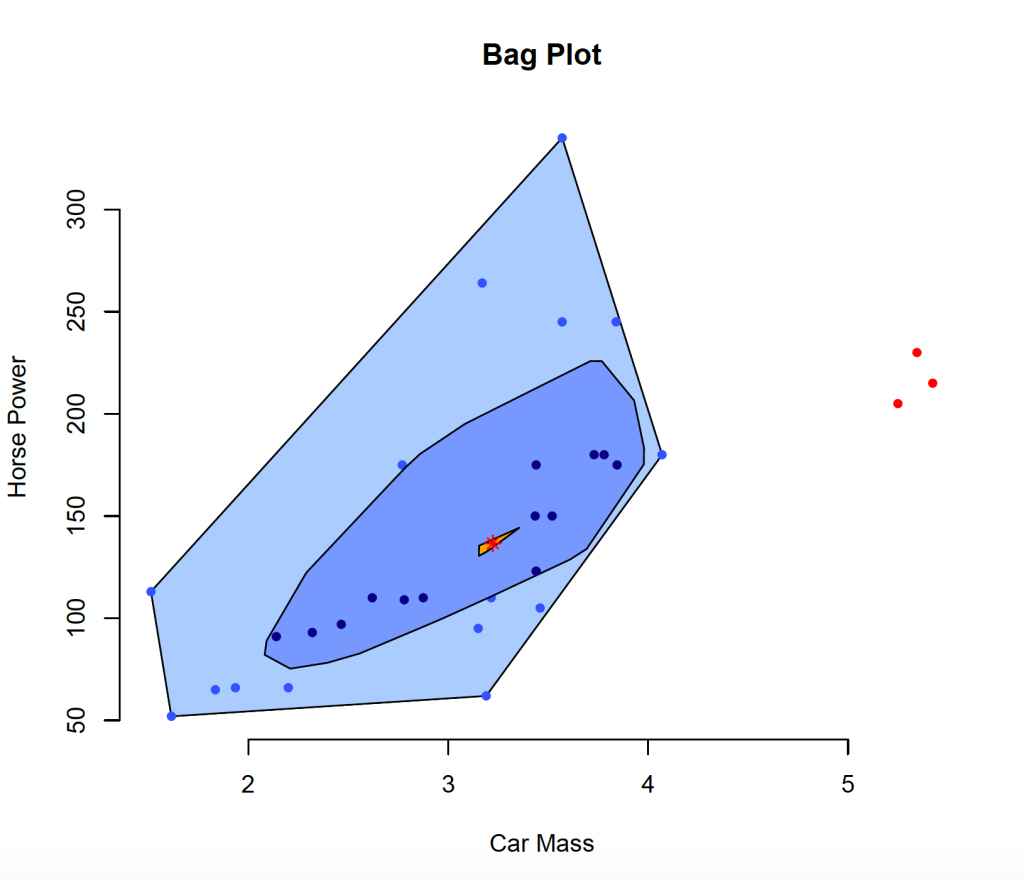
A bag plot is the scatterplot variant of a box and whisker plot where ‘bags’ correspond to the box in a box and whisker plot to illustrate outliers. To create a bag plot, use the aplpack library 1.
As illustration the ‘mtcars’ data frame that is part of base R is used. To show the first six observations (head) and the structure (str) of the data frame:
head(mtcars)
mpg cyl disp hp drat wt qsec vs am gear carb
Mazda RX4 21.0 6 160 110 3.90 2.620 16.46 0 1 4 4
Mazda RX4 Wag 21.0 6 160 110 3.90 2.875 17.02 0 1 4 4
Datsun 710 22.8 4 108 93 3.85 2.320 18.61 1 1 4 1
Hornet 4 Drive 21.4 6 258 110 3.08 3.215 19.44 1 0 3 1
Hornet Sportabout 18.7 8 360 175 3.15 3.440 17.02 0 0 3 2
Valiant 18.1 6 225 105 2.76 3.460 20.22 1 0 3 1
str(mtcars)
‘data.frame': 32 obs. of 11 variables:
$ mpg : num 21 21 22.8 21.4 18.7 18.1 14.3 24.4 22.8 19.2 …
$ cyl : num 6 6 4 6 8 6 8 4 4 6 …
$ disp: num 160 160 108 258 360 …
$ hp : num 110 110 93 110 175 105 245 62 95 123 …
$ drat: num 3.9 3.9 3.85 3.08 3.15 2.76 3.21 3.69 3.92 3.92 …
$ wt : num 2.62 2.88 2.32 3.21 3.44 …
$ qsec: num 16.5 17 18.6 19.4 17 …
$ vs : num 0 0 1 1 0 1 0 1 1 1 …
$ am : num 1 1 1 0 0 0 0 0 0 0 …
$ gear: num 4 4 4 3 3 3 3 4 4 4 …
$ carb: num 4 4 1 1 2 1 4 2 2 4 …
To create a bag plot:
library(aplpack)
bagplot(mtcars$wt, mtcars$hp, cex = 1, show.whiskers = FALSE, xlab = ‘Car Mass’, ylab = ‘Horse Power’, main = ‘Bag Plot’)
The inner dark-blue polygon is called the ‘bag’ and contains 50% of the data (similar to the box in a box plot). The fence (not show) is an area three times the bag. All data points outside the fence are outliers and indicated in red. The ‘loop’ (light-blue polygon) surrounds all data points that are not outliers (similar to the whiskers in a box plot).
